Download
1 / 79
2.27k likes | 4.25k Views
Introduction to Electromagnetic Theory Charges, Electric and Magnetic Fields. Assoc. Prof. Dr. Wanchai Pijitrojana Room 412-7 Research and Lab Bldg. pwanchai@engr.tu.ac.th. Objectives.

E N D
Introduction toElectromagnetic TheoryCharges, Electric and Magnetic Fields Assoc. Prof. Dr. WanchaiPijitrojana Room 412-7 Research and Lab Bldg. pwanchai@engr.tu.ac.th 1
Objectives • To provide an introductory course on classical electromagnetics, Maxwell’s equations, and electromagnetic fields in materials. • To prepare knowledge for students who want to continue in the fields of electrical engineering and electrophysics. 2
Textbooks by Richard E. Dubroff (Author), S. V. Marshall (Author), G. G. Skitek (Author) 3
James Clerk Maxwell James Clerk Maxwell, one of the world's greatest physicists, was Professor of Natural Philosophy at King's from 1860 to 1865, perhaps the most fertile years of his career. It was during this period that he demonstrated that magnetism, electricity and light were different manifestations of the same fundamental laws, and described all these, as well as radio waves, radar, and radiant heat, through his unique and elegant system of equations. These calculations were crucial to Albert Einstein in his production of the theory of relativity 40 years later, and led Einstein to comment that 'One scientific epoch ended and another began with James Clerk Maxwell'. Maxwell also made a major contribution to the understanding of colour vision and the first demonstration of colour photography. He produced notable work on the theory of rolling curves, on the composition of Saturn's rings, on the nature of gases and on electrical measurements. At King's the James Clerk Maxwell Building at the Waterloo Campus commemorates him, as does a chair in Physics named after him and a society for undergraduate physicists.
Electromagnetic Fields • Electromagnetics is the study of the effect of charges at rest and charges in motion. • Some special cases of electromagnetics: • Electrostatics: charges at rest • Magnetostatics: charges in steady motion (DC) • Electromagnetic waves: waves excited by charges in time-varying motion 6
Circuit Theory Electromagnetic Fields Maxwell’s equations Fundamental laws of classical electromagnetics Geometric Optics Electro-statics Magneto-statics Electro-magnetic waves Special cases Statics: Transmission Line Theory Input from other disciplines Kirchoff’s Laws 7
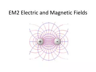
Electromagnetic Fields • transmitter and receiver • are connected by a “field.” 8
Electromagnetic Fields • When an event in one place has an effect on something at a different location, we talk about the events as being connected by a “field”. • A fieldis a spatial distribution of a quantity; in general, it can be either scalar or vector in nature. 9
Electromagnetic Fields • Electric and magnetic fields: • Are vector fields with three spatial components. • Vary as a function of position in 3D space as well as time. • Are governed by partial differential equations derived from Maxwell’s equations. 10
Electromagnetic Fields • A scalaris a quantity having only an amplitude (and possibly phase). • A vectoris a quantity having direction in addition to amplitude (and possibly phase). Examples: voltage, current, charge, energy, temperature Examples: velocity, acceleration, force 11
Electromagnetic Fields • Fundamental vector field quantities in electromagnetics: • Electric field intensity • Electric flux density (electric displacement) • Magnetic field intensity • Magnetic flux density units = volts per meter (V/m = kg m/A/s3) units = coulombs per square meter (C/m2 = A s /m2) units = amps per meter (A/m) units = teslas = webers per square meter (T = Wb/ m2 = kg/A/s3) 12
Electromagnetic Fields • Universal constants in electromagnetics: • Velocity of an electromagnetic wave (e.g., light) in free space (perfect vacuum) • Permeability of free space • Permittivity of free space: • Intrinsic impedance of free space: 13
Electromagnetic Fields • Relationships involving the universal constants: In free space: 14
sources Ji, Ki fields E, H Electromagnetic Fields • Obtained • by assumption • from solution to IE Solution to Maxwell’s equations Observable quantities 15
Maxwell’s Equations • Maxwell’s equations in integral form are the fundamental postulates of classical electromagnetics - all classical electromagnetic phenomena are explained by these equations. • Electromagnetic phenomena include electrostatics, magnetostatics, electromagnetostatics and electromagnetic wave propagation. • The differential equations and boundary conditions that we use to formulate and solve EM problems are all derived from Maxwell’s equations in integral form. 16
Maxwell’s Equations • Various equivalence principles consistent with Maxwell’s equations allow us to replace more complicated electric current and charge distributions with equivalent magnetic sources. • These equivalent magnetic sources can be treated by a generalization of Maxwell’s equations. 17
Maxwell’s Equations in Integral Form (Generalized to Include Equivalent Magnetic Sources) Adding the fictitious magnetic source terms is equivalent to living in a universe where magnetic monopoles (charges) exist. 18
Continuity Equation in Integral Form (Generalized to Include Equivalent Magnetic Sources) • The continuity equations are implicit in Maxwell’s equations. 19
S C dS S V dS Contour, Surface and Volume Conventions • open surface S bounded by • closed contour C • dS in direction given by • RH rule • volume V bounded by • closed surface S • dS in direction outward • from V 20
Electric Current and Charge Densities • Jc = (electric) conduction current density (A/m2) • Ji = (electric) impressed current density (A/m2) • qev = (electric) charge density (C/m3) 21
Magnetic Current and Charge Densities • Kc = magnetic conduction current density (V/m2) • Ki = magnetic impressed current density (V/m2) • qmv = magnetic charge density (Wb/m3) 22
Maxwell’s Equations - Sources and Responses • Sources of EM field: • Ki, Ji, qev, qmv • Responses to EM field: • E, H, D, B, Jc, Kc 23
Maxwell’s Equations in Differential Form (Generalized to Include Equivalent Magnetic Sources) 24
Continuity Equation in Differential Form (Generalized to Include Equivalent Magnetic Sources) • The continuity equations are implicit in Maxwell’s equations. 25
Electromagnetic Boundary Conditions Region 1 Region 2 26
Surface Current and Charge Densities • Can be either sources of or responses to EM field. • Units: • Ks - V/m • Js - A/m • qes - C/m2 • qms - W/m2 28
Electromagnetic Fields in Materials • In time-varying electromagnetics, we consider E and H to be the “primary” responses, and attempt to write the “secondary” responses D, B, Jc, and Kcin terms of E and H. • The relationships between the “primary” and “secondary” responses depends on the medium in which the field exists. • The relationships between the “primary” and “secondary” responses are called constitutive relationships. 29
Electromagnetic Fields in Materials • Most general constitutive relationships: 30
Electromagnetic Fields in Materials • In free space, we have: 31
Electromagnetic Fields in Materials • In a simple medium, we have: • linear(independent of field strength) • isotropic(independent of position within the medium) • homogeneous(independent of direction) • time-invariant(independent of time) • non-dispersive (independent of frequency) 32
Electromagnetic Fields in Materials • e = permittivity = ere0 (F/m) • m = permeability = mrm0(H/m) • s = electric conductivity = ere0(S/m) • sm = magnetic conductivity = ere0(W/m) 33
Phasor Representation of a Time-Harmonic Field • A phasor is a complex number representing the amplitude and phase of a sinusoid of known frequency. phasor frequency domain time domain 34
Phasor Representation of a Time-Harmonic Field • Phasors are an extremely important concept in the study of classical electromagnetics, circuit theory, and communications systems. • Maxwell’s equations in simple media, circuits comprising linear devices, and many components of communications systems can all be represented as linear time-invariant (LTI) systems. (Formal definition of these later in the course …) • The eigenfunctions of any LTI system are the complex exponentials of the form: 35
If the input to an LTI system is a sinusoid of frequency w, then the output is also a sinusoid of frequency w (with different amplitude and phase). Phasor Representation of a Time-Harmonic Field A complex constant (for fixed w); as a function of w gives the frequency response of the LTI system. 36
Phasor Representation of a Time-Harmonic Field • The amplitude and phase of a sinusoidal function can also depend on position, and the sinusoid can also be a vector function: 37
Phasor Representation of a Time-Harmonic Field • Given the phasor (frequency-domain) representation of a time-harmonic vector field, the time-domain representation of the vector field is obtained using the recipe: 38
Phasor Representation of a Time-Harmonic Field • Phasors can be used provided all of the media in the problem are linear no frequency conversion. • When phasors are used, integro-differential operators in time become algebraic operations in frequency, e.g.: 39
Time-Harmonic Maxwell’s Equations • If the sources are time-harmonic (sinusoidal), and all media are linear, then the electromagnetic fields are sinusoids of the same frequency as the sources. • In this case, we can simplify matters by using Maxwell’s equations in the frequency-domain. • Maxwell’s equations in the frequency-domain are relationships between the phasor representations of the fields. 40
Maxwell’s Equations in Differential Form for Time-Harmonic Fields 41
Maxwell’s Equations in Differential Form for Time-Harmonic Fields in Simple Medium 42
Circuit Theory Electrostatics as a Special Case of Electromagnetics Maxwell’s equations Fundamental laws of classical electromagnetics Geometric Optics Electro-statics Magneto-statics Electro-magnetic waves Special cases Statics: Transmission Line Theory Input from other disciplines Kirchoff’s Laws 43
Electrostatics • Electrostaticsis the branch of electromagnetics dealing with the effects of electric charges at rest. • The fundamental law of electrostatics is Coulomb’s law. 44
Electric Charge • Electrical phenomena caused by friction are part of our everyday lives, and can be understood in terms of electrical charge. • The effects of electrical charge can be observed in the attraction/repulsion of various objects when “charged.” • Charge comes in two varieties called “positive” and “negative.” 45
Electric Charge • Objects carrying a net positive charge attract those carrying a net negative charge and repel those carrying a net positive charge. • Objects carrying a net negative charge attract those carrying a net positive charge and repel those carrying a net negative charge. • On an atomic scale, electrons are negatively charged and nuclei are positively charged. 46
Electric Charge • Electric charge is inherently quantized such that the charge on any object is an integer multiple of the smallest unit of charge which is the magnitude of the electron charge e= 1.602 10-19C. • On the macroscopic level, we can assume that charge is “continuous.” 47
Coulomb’s Law • Coulomb’s law is the “law of action” between charged bodies. • Coulomb’s law gives the electric force between two point chargesin an otherwise empty universe. • A point charge is a charge that occupies a region of space which is negligibly small compared to the distance between the point charge and any other object. 48
Coulomb’s Law Q1 Q2 Unit vector in direction of R12 Force due to Q1 acting on Q2 49
Coulomb’s Law • The force on Q1due to Q2 is equal in magnitude but opposite in direction to the force on Q2 due to Q1. 50