Download
1 / 3
30 likes | 150 Views
0.03. 0.025. Euclidean DTW. CBF Dataset. 0.02. 0.015. 0.01. 0.005. 0. Out-of-Sample Error Rate. 0.5. Two-Pat Dataset. 0.4. 0.3. 0.2. 0.1. 0. 0. 1000. 2000. 3000. 4000. 5000. 6000. Increasingly Large Training Sets.

E N D
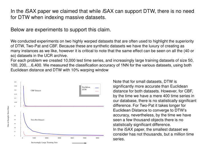
0.03 0.025 Euclidean DTW CBF Dataset 0.02 0.015 0.01 0.005 0 Out-of-Sample Error Rate 0.5 Two-Pat Dataset 0.4 0.3 0.2 0.1 0 0 1000 2000 3000 4000 5000 6000 Increasingly Large Training Sets In the iSAX paper we claimed that while iSAX can support DTW, there is no need for DTW when indexing massive datasets. Below are experiments to support this claim. We conducted experiments on two highly warped datasets that are often used to highlight the superiority of DTW, Two-Pat and CBF. Because these are synthetic datasets we have the luxury of creating as many instances as we like, however it is critical to note that the same effect can be seen on all the (40 or so) datasets in the UCR archive. For each problem we created 10,000 test time series, and increasingly large training datasets of size 50, 100, 200,…6,400. We measured the classification accuracy of 1NN for the various datasets, using both Euclidean distance and DTW with 10% warping window Note that for small datasets, DTW is significantly more accurate than Euclidean distance for both datasets. However, for CBF, by the time we have a mere 400 time series in our database, there is no statistically significant difference. For Two-Pat it takes longer for Euclidean Distance to converge to DTW’s accuracy, nevertheless, by the time we have seen a few thousand objects there is no statistically significant difference. In the iSAX paper, the smallest dataset we consider has not thousands, but a million time series.
The intuition behind the idea that iSAX can support DTW indexing is simple. We can build bounding envelopes U and L around the query time series Q. We then have a lower bound between the query and any time series C. This lower bound, the LB_Keogh is simply the green hatch lines in the below figure. Having built the envelope for just the query, the only thing we need do is modify the iSAX MINDIST function. We convert both the U and L envelopes into iSAX words, but we don’t normalize them first. Now, in the iSAX MINDIST function, instead of comparing the symbols of the query to the symbols of the candidate match C, we compare the symbols of the envelope to the symbols of the candidate match. If the ith symbol of C falls in between the ith symbols of U and L, the function should return zero, otherwise it should return the min(dist(Ci,Li), dist(Ci,Ui)) Given this admissible iSAX lower bound of DTW, with just a few minor bookkeeping changes, the iSAX indexing code can be used 3 C 2 Q 1 U L 0 -1 -2 Q -3 0 2 4 6 8 10 12 14 16 0 2 4 6 8 10 12 14 16 0 2 4 6 8 10 12 14 16
C C Q U L Q LB_Keogh Review of LB_Keogh See Keogh, E. (2002). Exact indexing of dynamic time warping. In 28th International Conference on Very Large Data Bases. Hong Kong. pp 406-417. U Ui = max(qi-r : qi+r) Li = min(qi-r : qi+r) L Q Sakoe-Chiba Band Envelope-Based Lower Bound