Download
1 / 19
190 likes | 339 Views
CPSC 422 Review Of Probability Theory. Uncertainty. Let action A t = leave for airport t minutes before flight Will A t get me there on time? Problems: partial observability (road state, other drivers' plans, etc.) noisy sensors (traffic reports)

E N D
CPSC 422Review Of Probability Theory
Uncertainty Let action At = leave for airport t minutes before flight Will At get me there on time? Problems: • partial observability (road state, other drivers' plans, etc.) • noisy sensors (traffic reports) • uncertainty in action outcomes (flat tire, etc.) • immense complexity of modeling and predicting traffic Hence a purely logical approach either • risks falsehood: “A25 will get me there on time”, or • leads to conclusions that are too weak for decision making: “A25 will get me there on time if there's no accident on the bridge and it doesn't rain and my tires remain intact etc etc.” (A1440 might reasonably be said to get me there on time but I'd have to stay overnight in the airport …)
Methods for handling uncertainty • Default or nonmonotonic logic: • Assume my car does not have a flat tire • Assume A25 works unless contradicted by evidence • Issues: What assumptions are reasonable? How to handle contradiction? • Rules with fudge factors: • A25 |→0.3 get there on time • Sprinkler |→0.99WetGrass • WetGrass |→0.7Rain • Issues: Problems with combination, e.g., Sprinkler causes Rain?? • Probability • Model agent's degree of belief that: • Given the available evidence, A25 will get me there on time with probability 0.04
Probability Probabilistic assertions summarize effects of • laziness: failure to enumerate exceptions, qualifications, etc. • E.g. A25 will do if there is no traffic, no constructions, no flat tire…. • ignorance: lack of relevant facts, initial conditions, etc. Subjective probability: • Probabilities relate propositions to agent's own state of knowledge • e.g., P(A25 | no reported accidents) = 0.06 These are not assertions about the world Probabilities of propositions change with new evidence: • e.g., P(A25 | no reported accidents, 5 a.m.) = 0.15
Probability theory • System of axioms and formal operations for sound reasoning under uncertainty • Basic element: random variable, with an set of possible values (domain) • Boolean: e.g., Cavity (do I have a cavity or not?), Toothache (do I have a toothache or not), Catch (does the dentist’s probe catch in my tooth or not) • We will abbreviate: P(Var = true) as P(var). P(Var = false) as P(var) • Discrete: e.g., Weather is one of <sunny, rainy, cloudy, snow> • We will abbreviate: P(Var = value) as P(value) • Continuous: e.g., Temperature-in-January is defined by a probability density function (e.g. Gaussian distribution)
Probability theory • Prior or unconditionalprobabilities of propositions, e.g. • P(cavity) = 0.1 correspond to belief on the state of the world prior to arrival of any (new) evidence • Conditional Probability specifies how to revise beliefs based on new information: conditional or posterior probabilities, e.g., • P(cavity | toothache) = • P(cavity | toothache, catch ) = • Probability distribution gives values for all possible assignments: • P(Weather) = <0.72, 0.1, 0.08, 0.1> (normalized, i.e., sums to 1) • Atomic event: A conjunction of assignments <Variablei, valueij> for all the variables in my domain (we’ll forget about Weather for now) • Toothache = true Cavity = true Catch = false • Joint Probability Distribution (JPD) for a set of random variables • probability of every atomic event on those random variables
Joint Probability Distribution • Example: P(Toothache,Cavity, Catch) = a 2 × 2 × 2 matrix of values:
Conditional probability • Definition of conditional probability: • P(a | b) = P(a b) / P(b) if P(b) > 0 • Product rule gives an alternative, more intuitive formulation: • P(a b) = P(a | b) P(b) = P(b | a) P(a) • A general version holds for whole distributions, e.g., • P(Weather,Cavity) = P(Weather | Cavity) P(Cavity) (View as a set of 4 × 2 equations, not matrix mult.) • Chain rule is derived by successive application of product rule: P(X1, …,Xn) = = P(X1,...,Xn-1) P(Xn | X1,...,Xn-1) = P(X1,...,Xn-2) P(Xn-1 | X1,...,Xn-2) P(Xn | X1,...,Xn-1) = …. = P(X1 | X2)…P(X1,...,Xn-2) P(Xn-1 | X1,...,Xn-2) P(Xn | X1,.,Xn-1) = ∏ni= 1P(Xi | X1, … ,Xi-1)
Basic Probabilistic Inference (inference by enumeration) • Every question about a domain can be answered by its joint distribution : • For any proposition φ, sum the atomic events where it is true • P(cavity or toothache) = .108+.012+.072+.008+.016+.064 = 0.28
Inference by enumeration • Can also compute conditional probabilities: P(cavity | toothache) =
Inference by enumeration • Can also compute conditional probabilities: P(cavity | toothache) = P(cavity toothache) / P(toothache) = 0.016+0.064 = 0.4 0.108 + 0.012 + 0.016 + 0.064
Normalization • Denominator can be viewed as a normalization constant α P(Cavity | toothache) = P(Cavity,toothache) |P(toothache) = αP(Cavity,toothache) = α [P(Cavity,toothache,catch) + P(Cavity,toothache,catch)] = α [<0.108, 0.016> + <0.012, 0.064>] = α <0.12, 0.08> = <0.6, 0.4>
Inference by enumeration, contd. • Typically, given a set of domain variables X, we are are interested in the posterior joint distribution of • the query variablesY (subset of X) • given specific values e for the evidence variablesE (subset of X) • Let the hidden variables be H = X - Y – E = [Hi,…Hj] • General idea: compute distribution on query variable Y by fixing evidence variables and summing over hidden variables • P(Y|E) = ∑H1..... ∑HjP(H1,…,Hj,Y,E) • The terms in the summation are joint entries because Y, E and H together exhaust the set of random variables • Obvious problems: • Worst-case time complexity O(dn) where d is the size of largest domain • Space complexity O(dn) to store the joint distribution • How to find the numbers for O(dn) entries?
Independence • A and B are independent iff: P(A|B) = P(A) or P(B|A) = P(B) or P(A, B) = P(A) P(B) • That is new evidence B (or A) does not affect current belief in A (or B) • Ex:P(Toothache, Catch, Cavity, Weather) = P(Toothache, Catch, Cavity) P(Weather) • JPD requiring 32 entries is reduced to two smaller ones (8 and 4)
Independence • for n independent biased coins, O(2n)→O(n) • Absolute independence powerful but rare • Dentistry is a large field with hundreds of variables, none of which are independent. What to do?
Conditional independence • If I have a cavity, the probability that the probe catches in it doesn't depend on whether I have a toothache: (1) P(catch | toothache, cavity) = P(catch | cavity) • The same independence holds if I haven't got a cavity: (2) P(catch | toothache,cavity) = P(catch | cavity) • Catch is conditionally independent of Toothache given Cavity: P(Catch | Toothache,Cavity) = P(Catch | Cavity)
Conditional independence contd. • Write out full joint distribution using chain rule: P(Toothache, Catch, Cavity) = P(Toothache | Catch, Cavity) P(Catch, Cavity) = P(Toothache | Catch, Cavity) P(Catch | Cavity) P(Cavity) = P(Toothache | Cavity) P(Catch | Cavity) P(Cavity) I.e., 2 + 2 + 1 = 5 independent numbers • In most cases, the use of conditional independence reduces the size of the representation of the joint distribution from exponential in n to linear in n. • Conditional independence is our most basic and robust form of knowledge about uncertain environments. • Bayesian networks are a formalism to reason under uncertainty specifically designed to exploit this knowledge
Bayes' Rule • Product rule P(ab) = P(a | b) P(b) = P(b | a) P(a) Bayes' rule: P(a | b) = P(b | a) P(a) / P(b) • or in distribution form P(Y|X) = P(X|Y) P(Y) / P(X) = αP(X|Y) P(Y) • Useful for assessing diagnostic probability from causal probability: • P(Cause|Effect) = P(Effect|Cause) P(Cause) / P(Effect) • E.g., let m be meningitis, s be stiff neck: P(m|s) = P(s|m) P(m) / P(s) = 0.8 × 0.0001 / 0.1 = 0.0008 • Note: posterior probability of meningitis still very small!
Bayes' Rule and conditional independence P(Cavity | toothache catch) = P(toothache catch | Cavity) P(Cavity) |P(toothache catch) = αP(toothache catch | Cavity) P(Cavity) = αP(toothache | Cavity) P(catch | Cavity) P(Cavity) • This is an example of a naïve Bayes model: P(Cause, Effect1, … ,Effectn) = P(Cause) πiP(Effecti|Cause) • Total number of parameters is linear in n