Download
1 / 37
370 likes | 493 Views
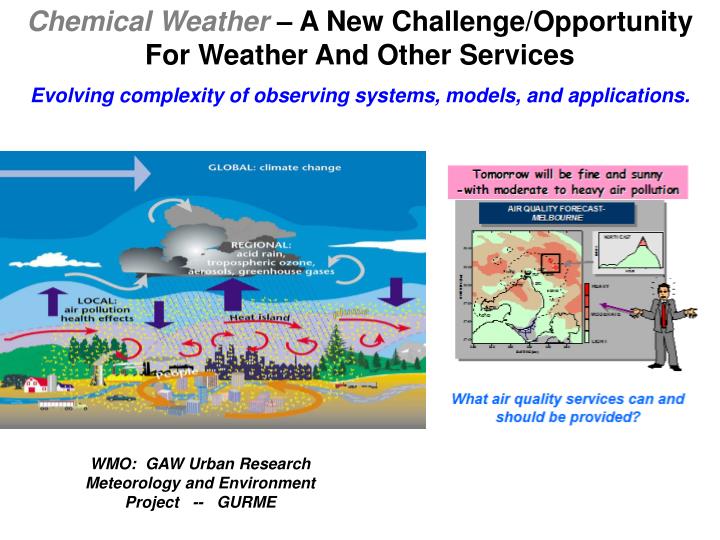
Chemical Weather – A New Challenge/Opportunity For Weather And Other Services Evolving complexity of observing systems, models, and applications. WMO: GAW Urban Research Meteorology and Environment Project -- GURME. Slide provided by Paula Davidson.

E N D
Chemical Weather – A New Challenge/Opportunity For Weather And Other Services Evolving complexity of observing systems, models, and applications. WMO: GAW Urban Research Meteorology and Environment Project -- GURME
Forecast Skill By Region Of NOAA’s Ozone And PM2.5 Predictions Design target Fraction Correct O3 PM2.5 Operational Testing Slide provided by Paula Davidson
Evaluation Discrete Forecast / Evaluation Observed vs. Forecast Max. 8 hr. Concentration Example of strict grid-cell to monitor matching CONUS Forecasts for the Summer (J, J, A) Eder et al., 2009
Current Evaluation Approach The statistics below are based on using all8 monitors in the Charlotte MSA with the monitors matcheddirectly with their grid cell. Period: 1 May – 30 Sept. 2007 n = 1207 MB = 2.1 ppb; NMB = 3.3% RMSE = 12.0 ppb; NME = 16.8% r = 0.63 Eder et al., 2009
Modified Evaluation Approach - Step 1 The statistics below are based on the max. of the 8 monitors and the max. of 8 grid cells in the Charlotte MSA, where monitors are not matched with their grid cell. Period: 1 May – 30 Sept. 2007 n = 153 MB = -0.8 ppb; NMB -1.1% RMSE = 10.5 ppb; NME = 11.8% r = 0.73 Eder et al., 2009
Modified Evaluation Approach - Step 2 The statistics below are based on the maximum of the 8 monitors and maximum of all 103 model grid cells in the Charlotte MSA, where the monitors are not matched with their grid cell. Period: 1 May – 30 Sept. 2007 n = 153 MB = 3.1 ppb; NMB = 4.4% RMSE = 11.0 ppb; NME = 13.1% r = 0.74 Eder et al., 2009
Evaluation Adaptation This modified, somewhat more relaxed evaluation approach results in “improved” statistics when compared to the more rigid observation vs. grid cell approach. ●We will demonstrate this approach using both: [O3]AQI Eder et al., 2009
Modified Evaluation Approach - Step 3 We can take the last approach and convert the concentrations to AQI values. Period: 1 May – 30 Sept. 2007 n = 153 MB = 6.7; NMB = 9.3% RMSE = 22.0; NME = 25.1% r = 0.74 Eder et al., 2009
Category Hit Rate: where i is the AQI index (1, 2, 3, 4, 5) category or the color scheme (green, yellow, orange, red, purple), and is the forecast instances in the i th category and is the number of observed instances in the i th category. NAQFC Categorical Performance vs.Human Forecast • Exceedance Hit Rate: • where N fo is the number of both observed and forecast • exceedances (AQI ≥ 3), Nois the number of observed, but not forecast exceedances. • Exceedance False Alarm Rate: • where Nf is the number of forecast but not observed exceedances (AQI ≥3), Nfois the number of both observed and forecast exceedances. Eder et al., 2009
NAQFC Performance compared with Human Forecast* Summer 2007 * Provided by NC Department of Environmental and Natural Resources Eder et al., 2009
NAQFC Categorical Performance vs.Human Forecast Exceedance Hit Rate Exceedance False Alarm Rate Human NAQFC Because the NAQFC is positively biased, it tends to capture a higher percentage of exceedance hit rates, but this also results in a higher percentage of false alarm rates. Eder et al., 2009
Intensive field experiments provide opportunities for comprehensive evaluations Current CTMs Do Have Appreciable Skills In Predicting A Wide Variety Of Parameters INTEX B – STEM Forecasts C130 DC8 DC8 C130
Ensemble Forecasting of Air Quality OZONE *Persistence * Single Forward Model w/o assimilation * Ensemble forecast (8 models) w/o assimilation (further improvements with bias corrections based on obs) McKeen et al., JGR, 2005
Ensemble Forecast Evaluation During Major Field ExperimentsPM2.5 Remains a Challenge O3 NEAQS-2004 PM2.5 TexAQS-2006 McKeen et al., JGR, 2005 & 2009
Optimal analysis state Chemical kinetics Observations CTM Data Assimilation Aerosols Emissions Regional-Scale Chemical Analysis for Air Quality Modeling: A Closer Integration Of Observations And Models Transport Meteorology • Improved: • forecasts • science • field experiment design • models • emission estimates • S/R relationships
Data assimilation methods • “Simple” data assimilation methods • Optimal Interpolation (OI) • 3-Dimensional Variational data assimilation (3D-Var) • Kriging • Advanced data assimilation methods • 4-Dimensional Variational data assimilation (4D-Var) • Kalman Filter (KF) - Many variations, e.g. Ensemble Kalman Filter (EnFK)
Challenges in chemical data assimilation • A large amount of variables (~300 concentrations of various species at each grid points) • Memory shortage (check-pointing required) • Various chemical reactions (>200) coupled together (lifetimes of species vary from seconds to months) • Stiff differential equations • Chemical observations are very limited, compared to meteorological data • Information should be maximally used, with least approximation • Highly uncertain emission inventories • Inventories often out-dated, and uncertainty not well-quantified
Assimilation of MODIS AOD to Produce Constrained Fields for Climate Calculations How to optimally adjust individual aerosol quantities given AOD (sulfate, BC, OC, dust, sea salt)? - AOD by itself not unique - Fine mode fraction helps - SSA gives info to adjust abs vs scat. Technique: Collins, W. D., et al. (2001),, JGR, 106, 7313-7336 W - Assimilation w/o - “ Chul et al., JGR, 2005 Adhikary et al., 2007,2008
Impact of Daily MODIS Assimilation on Predicted PM 2.5 at HCO Start of assimilation Adhikary et al., 2007,2008
ARW-WRF/Chem and the Gridpoint Statistical Interpolation (GSI) Analysis System (3dVar) Now building a 4dvar system O3 Forecast period Control PM2.5 Bias RMSE R Grell et al., 2009
Assimilation of ICARTT Ozone Observations -- Assessing Information Content
Assimilation Produces An Optimal State Space the importance of measurements above the surface! with assimilation w/o assimilation Ozone predictions Example July 20, 2004 with w/o assimilation Information below 4 km most important Region-mean profile Chai et al., JGR 2007
Ensemble-based chemical data assimilation techniques can complement the variational tools • Motivation: • Ensemble-based d.a. generate a statistical sample of analyses • Optimal state estimation applied to each member • Can deal effectively with nonlinear dynamics • Explicitly propagate (approximations of) the error statistics • Complement variational techniques • Issues: • Initialization of the ensemble • Rank-deficient covariance matrix • Contributions: • Models of background error covariance • Calculation of TESVs for reactive flows • Targeted observations using TESVs • Ensemble-based assimilation results
Challenges for reanalysis and forecasting appear to be different …. 4D-var and EnKF show promise for reanalysis Sandu et al., Quart. J. Roy. Met. Soc, 2007
Challenges for reanalysis and forecasting appear to be different …. 4D-var and EnKF show promise for reanalysis but more work is needed to impact forecasts Sandu et al., QJRMS, 2007
Advanced Data Assimilation Techniques Provide Data Fusion and Optimal Analysis Frameworks Example 4dVar: Cost function Observations information consistent with reality Current knowledge of the state Model information consistent with physics/chemistry The system is very under-determined – need to combine heterogeneous data sources with limited spatial/temporal information
Estimation of B and O criticalNMC method (B) • Substitute model background errors with the differences between 24hr, 48 hr, 72 hr forecasts verifying at the same time • Calculate the model background error statistics in three directions separately • Equivalent sample number: 811,890
NMC method results Vertical correlation Horizontal correlation l=2.5km l=270m
Observational error • Observational Error: • Representative error • Measurement error • Observation Inputs • Averaging inside 4-D grid cells • Uniform error (8 ppbv)
In AQ Predictions Emissions Are A Major Source Of Uncertainty – Data Assimilation Can Produce Optimal Estimates (Inverse Applications) Li et al., Atmos. Env., 2007
Rapid Updates of Emissions Are Needed Scaling factors
Phenological models Many Meteorological Services Already Supply Operational Chemical Weather Products (e.g., FMI) Fire Assimilation System Satellite observations Final AQ products Phenological observations SILAM AQ model Aerobiological observations EVALUATION: NRT model-measurement comparison Physiography, forest mapping Assimilation HIRLAM NWP model Aerobiological observations Online AQ monitoring UN-ECE CLRTAP/EMEP emission database Meteorological data: ECMWF Real-time data needs!
Section 13Developing a Forecasting Program Understanding Users’ Needs Understanding the Processes that Control Air Quality Choosing Forecasting Tools Data Types, Sources, and Issues Forecasting Protocol Forecast Verification