Download
1 / 13
130 likes | 159 Views
Explore the concepts of starlight and brightness through magnitude calculations, inverse square law, absolute and apparent magnitudes, distance modulus, and spectral classification in astronomy. Learn about the color index, Wien's Law, spectral types, and factors influencing star properties.

E N D
Apparent brightness 2nd century BC Hipparchus devised 6 categories of brightness. In 1856 Pogson discovered that there is a 1:100 ratio in brightness between magnitude 1 and 6 mathematical tools are possible. m1-m2 = 2.5 log (I2/I1) m1 and m2 are visual magnitudes, I1 and I2 are brightness.
Example Vega is 10 times brighter than a magnitude 1 star I2/I1 = 10. m1 = 1 2.5 log (I2/I1) = 2.5 1 - m2 = 2.5 m2 = -1.5 Using the same calculations we can find that Sun : -26.5 Full Moon : -12.5 Venus : -4.0 Mars : -2.0
Inverse Square Law Sun is very bright, because it is very near to us, but is the Sun really a “bright” star. The amount of light we receive from a star decreases with distance from the star.
Absolute Magnitude • If two pieces of information is known, we can find the absolute magnitude, M, of a star: • Apparent magnitude, m • Distance from us. • Example: • Take the Sun, 1AU = 1 / 200,000 parsecs away from us. • At 10 parsecs the Sun will be (2,000,000)2 times less bright. • log(2,000,0002) = 31.5 magnitudes dimmer • -26.5 (apparent) + 31.5 = 5 (absolute) • We define the absolute magnitude as the magnitude of a star as if it were 10pc away from us.
Distance modulus m –M : distance modulus Example: We have a table in our hands with distance moduli and we need to find the actual distances to the stars. How do we proceed?? Distance modulus = 10 means 10(10/2.5) = 10,000 times dimmer than the apparent magnitude (10,000) = 1002 (inverse square law) 10 pc x 100 1000 pc away
20 Brightest Stars Common Luminosity Distance Spectral Proper Motion R. A. Declination Name Solar Units LY Type arcsec / year hours min deg min Sirius 40 9 A1V 1.33 06 45.1 -16 43 Canopus 1500 98 F01 0.02 06 24.0 -52 42 Alpha Centauri 2 4 G2V 3.68 14 39.6 -60 50 Arcturus 100 36 K2III 2.28 14 15.7 +19 11 Vega 50 26 A0V 0.34 18 36.9 +38 47 Capella 200 46 G5III 0.44 05 16.7 +46 00 Rigel 80,000 815 B8Ia 0 05 12.1 -08 12 Procyon 9 11 F5IV-V 1.25 07 39.3 +05 13 Betelgeuse 100,000 500 M2Iab 0.03 05 55.2 +07 24 Achernar 500 65 B3V 0.1 01 37.7 -57 14 Beta Centauri 9300 300 B1III 0.04 14 03.8 -60 22 Altair 10 17 A7IV-V 0.66 19 50.8 +08 52 Aldeberan 200 20 K5III 0.2 04 35.9 +16 31 Spica 6000 260 B1V 0.05 13 25.2 -11 10 Antares 10,000 390 M1Ib 0.03 16 29.4 -26 26 Pollux 60 39 K0III 0.62 07 45.3 +28 02 Fomalhaut 50 23 A3V 0.37 22 57.6 -29 37 Deneb 80,000 1400 A2Ia 0 20 41.4 +45 17 Beta Crucis 10,000 490 B0.5IV 0.05 12 47.7 -59 41 Regulus 150 85 B7V 0.25 10 08.3 +11 58
Wien’s Law Wien’s Law: 1/T The higher the temperature The lower is the wavelengths The “bluer” the star.
Temperature Dependence Question: Where does the temperature dependence of the spectra come from? Answer: Stars are made up of different elements at different temperatures and each element will have a different strength of absorption spectrum. Take hydrogen; at high temperatures H is ionized, hence no H-lines in the absorption spectrum. At low T, H is not excited enough because there are not enough collisions.
Color Index To categorize the stars correctly, we pass the light through filters. B is a blue filter, V is a visible filter. Hot stars have a negative B-V color index. Colder stars have a positive B-V color index.
Spectral Types We now know that we can find the temperature of a star from its color. To categorize the “main sequence” stars we have divided the colors into seven spectral classes: Color Class solar masses solar diameters Temperature ---------------------------------------------------------------------------------- bluest O 20 – 100 12 - 25 40,000 bluish B 4 - 12 4 - 12 18,000 blue-white A 1.5 - 4 1.5 - 4 10,000 white F 1.05 - 1.5 1.1 - 1.5 7,000 yellow-white G 0.8 - 1.05 0.85 - 1.1 5,500 orange K 0.5 - 0.8 0.6 - 0.85 4,000 red M 0.08 - 0.5 0.1 - 0.6 3,000 Also each spectral class is divided into 10: Sun G2
What do we learn? Temperature and Pressure: ionization of different atoms to different levels. Chemical Composition: Presence and strength of absorption lines of various elements in comparison with the properties of the same elements under laboratory conditions gives us the composition of elements of a star. Radial velocity: We can measure a star’s radial velocity by the shift of the absorption lines using Doppler shift. Rotation speed: Broadens the absorption lines, the broader the lines, the higher the rotation speed. Magnetic field: With strong magnetic fields, the spectral lines are split into two or more components.