Download
1 / 37
380 likes | 591 Views
Introduction to Artificial Intelligence (G51IAI). Dr Matthew Hyde Neural Networks. More precisely: “ Artificial Neural Networks” Simulating, on a computer, what we understand about neural networks in the brain. Lecture Outline. Recap on perceptrons Linear Separability

E N D
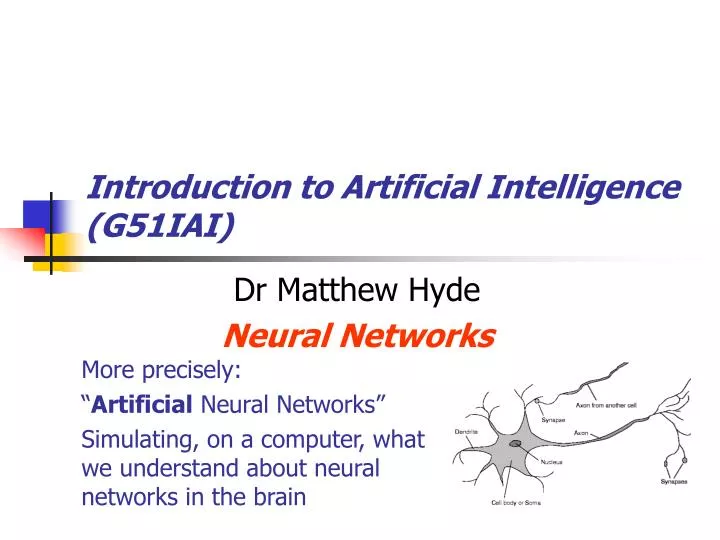
Introduction to Artificial Intelligence (G51IAI) Dr Matthew Hyde Neural Networks • More precisely: • “Artificial Neural Networks” • Simulating, on a computer, what we understand about neural networks in the brain
Lecture Outline • Recap on perceptrons • Linear Separability • Learning / Training • The Neuron’s Activation Function
Recap from last lecture • A ‘Perceptron’ • Single layer NN (one neuron) • Inputs can be any number • Weights on the edges • Output can only be 0 or 1 5 0.5 θ = 6 6 2 Z 0 or 1 3 -3
AND function, and OR function AND XOR These are called “truth tables”
AND function, and OR function AND XOR These are called “truth tables”
Important!!! • You can represent any truth table graphically, as a diagram • The diagram is 2-dimensional if there are two inputs • 3-dimensional if there are three inputs • Examples on the board in the lecture, and in the handouts
3 Inputs means 3-dimensions 0,1,0 1,1,0 0,1,1 1,1,1 Y axis X axis Z axis 0,0,0 1,0,0 0,0,1 1,0,1
Linear Separability in 3-dimensions Instead of a line, the dots are separated by a plane
0,1 0,1 1,1 1,1 0,0 1,0 XOR 0,0 1,0 XOR AND Minsky & Papert AND • Functions which can be separated in this way are called Linearly Separable • Only linearly Separable functions can be represented by a Perceptron
Examples – Handout 3 • Linear Separability • Fill in the diagrams with the correct dots • black or white, for an output of 1 or 0
Simple Networks AND X 1 θ=1.5 1 Y -1 Both of these represent the AND function. It is sometimes convenient to set the threshold to zero, and add a constant negative input 1.5 X θ=0 1 1 Y
0,1 1,1 AND 0,0 1,0 Training a NN AND
Randomly Initialise the Network • We set the weights randomly, because we do not know what we want it to learn. • The weights can change to whatever value is necessary • It is normal to initialise them in the range [-1,1]
Randomly Initialise the Network -1 0.3 0.5 X θ=0 Y -0.4
Learning While epoch produces an error Present network with next inputs (pattern) from epoch Err = T – O If Err <> 0 then Wj = Wj + LR * Ij * Err End If End While Get used to this notation!! Make sure that you can reproduce this pseudocode AND understand what all of the terms mean
Epoch • The ‘epoch’ is the entire training set • The training set is the set of four input and output pairs DESIRED OUTPUT INPUT
The learning algorithm DESIRED OUTPUT INPUT Input the first inputs from the training set into the Neural Network What does the neural network output? Is it what we want it to output? If not then we work out the error and change some weights
First training step • Input 1, 1 • Desired output is 1 • Actual output is 0 -1 0.3 0.5 1 θ=0 -0.3 + 0.5 + -0.4 = -0.2 1 -0.4 = Output of 0
First training step • We wanted 1 • We got 0 • Error = 1 – 0 = 1 While epoch produces an error Present network with next inputs (pattern) from epoch Err = T – O If Err <> 0 then Wj = Wj + LR * Ij * Err End If End While If there IS an error, then we change ALL the weights in the network
If there is an error, change ALL the weights • Wj = Wj + ( LR * Ij * Err ) • New Weight = Old Weight + (Learning Rate * Input Value * Error) • New Weight = 0.3 + (0.1 * -1 * 1) = 0.2 -1 0.3 0.2 0.5 1 θ=0
If there is an error, change ALL the weights • Wj = Wj + ( LR * Ij * Err ) • New Weight = 0.5 + (0.1 * 1 * 1) = 0.6 -1 0.2 0.5 0.6 1 θ=0 -0.4 1
Effects of the first change • The output was too low (it was 0, but we wanted 1) • Weights that contributed negatively have reduced • Weights that contributed positively have increased • It is trying to ‘correct’ the output gradually -1 -1 0.2 0.3 0.5 0.6 X X θ=0 θ=0 Y Y -0.3 -0.4
Epoch not finished yet • The ‘epoch’ is the entire training set • We do the same for the other 3 input-output pairs DESIRED OUTPUT INPUT
The epoch is now finished • Was there an error for any of the inputs? • If yes, then the network is not trained yet • We do the same for another epoch, from the first inputs again
The epoch is now finished • If there were no errors, then we have the network that we want • It has been trained While epoch produces an error Present network with next inputs (pattern) from epoch Err = T – O If Err <> 0 then Wj = Wj + LR * Ij * Err End If End While
Effect of the learning rate • Set too high • The network quickly gets near to what you want • But, right at the end, it may ‘bounce around’ the correct weights • It may go too far one way, and then when it tries to compensate it will go too far back the other way Wj = Wj + ( LR * Ij * Err )
0,1 1,1 0,0 1,0 AND Effect of the learning rate • Set too high • It may ‘bounce around’ the correct weights
Effect of the learning rate • Set too low • The network slowly gets near to what you want • It will eventually converge (for a linearly separable function) • but that could take a long time • When setting the learning rule, you have to strike a balance between speed and effectiveness Wj = Wj + LR * Ij * Err
Expanding the Model of the Neuron: Outputs other than ‘1’ Output is 1 or 0 It doesn’t matter about how far over the threshold we are X1 θ = 5 2 20 Y1 -5 -10 1 X2 θ = 2 -2 θ = 9 1 -4 Z Y2 5 0 1 1 X3 3 1 2 1 6 θ = 0
Example from last lecture Left wheel speed Right wheel speed ... ... The speed of the wheels is not just 0 or 1
Expanding the Model of the Neuron: Outputs other than ‘1’ • So far, the neurons have only output a value of 1 when they fire. • If the input sum is greater than the threshold the neuron outputs 1. • In fact, the neurons can output any value that you want.
Modelling a Neuron • aj : Input value (output from unit j) • wj,i : Weight on the link from unit j to unit i • ini : Weighted sum of inputs to unit i • ai : Activation value of unit i • g : Activation function
Activation Functions • Stept(x) = 1 if x >= t, else 0 • Sign(x) = +1 if x >= 0, else –1 • Sigmoid(x) = 1/(1+e-x) • aj : Input value (output from unit j) • ini : Weighted sum of inputs to unit i • ai : Activation value of unit i • g : Activation function
Summary • Linear Separability • Learning Algorithm Pseudocode • Activation function (threshold, sigmoid, etc)