Download
1 / 85
850 likes | 868 Views
This article explains the Q-Vector approach in Quasi-geostrophic theory for analyzing vertical motions and forcing in atmospheric systems. It covers the strengths and weaknesses of Q-Vector analysis and provides a case study for practical application.

E N D
Q-G Theory:Using the Q-Vector Patrick Market Department of Atmospheric Science University of Missouri-Columbia
Introduction • Q-G forcing for w • Vertical motions (particularly in an ETC) complete a secondary ageostrophic circulation forced by geostrophic and hydrostatic adjustments on the synoptic-scale. • Evaluation • Traditional • Laplacian of thickness advection • Differential vorticity advection • PIVA/NIVA (Trenberth Approximation) • Q-vector
Q-vector Strengths • Eliminates competition between terms in the Q-G w equation • Unlike PIVA/NIVA, deformation is retained as a forcing mechanism • Q-vectors are proportional in strength and lie along the low level Vag. • Analysis of Q-vectors with isentropes can reveal areas of frontogenesis/frontolysis. • Only one isobaric level is needed to compute forcing.
Q-vector Weaknesses • Diabatic heating/cooling are neglected • Variations in f are neglected • Variations in static stability are neglected • w is still not calculated; its forcing is • Although one may employ a single level for the process, layers are thought to be better for Q evaluation • So, which layer to use?
Q-vector: Choosing a layer… • RECALL: Q-G forcing for w • Vertical motions complete a secondary ageostrophic circulation… • Inertial-advective adjustments with the ULJ • Isallobaric adjustments with the LLJ • Deep layers can be useful • Max vertical motion should be near LND (~550 mb) • Ideally that layer will be included
Q-vector: Choosing a layer… • Avoid very low levels (PBL) • Friction • Radiative/sensible heating/cooling • Look • low enough to account for CAA/WAA • deep enough to account for vertical change in vorticity advection • Typical layer: 400-700 mb • Brackets LND (~550 mb) • Deep enough to • Capture low level thermal advection • Significant differential vorticity advection
A Definition of Q • Q is the time rate of change of the potential temperature gradient vector of a parcel in geostrophic motion (after Thaler)
Simple Example 1 Z • True gradient vector points L H • Equivalent barotropic environment (after Thaler) T Z+DZ T+DT Z+2DZ
Simple Example 2 (after Thaler) Z T Z+DZ T+DT Z+2DZ
A Purpose for Q • If Q exists, then the thermal gradient is changing following the motion… • So… thermal wind balance is compromised • So… the thermal wind is no longer proportional to the thickness gradient • So… geostrophic and hydrostatic balance are compromised • So… forcing for vertical motion ensues as the atmosphere seeks balance
Known Behaviors of Q • Q often points along Vag in the lower branch of a transverse, secondary circulation • Q often proportional to low-level |Vag| • Q points toward rising motion • Q plotted with a field of q can reveal regions of F • FQ-G • Q points toward warm air – frontogenesis • Q points toward cold air – frontolysis
Q Components • Qn – component normal to q contours • Qs – component parallel to q contours q Qn Q q+Dq Qs q+2Dq
Aspects of Qn • Indicates whether geostrophic motion is frontolytic or frontogenetic • Qn points ColdWarm Frontogenesis • Qn points WarmCold Frontolysis • For f=f0, the geostrophic wind is purely non-divergent • Q-G frontogenesis is due entirely to deformation
Aspects of Qs • Determines if the geostrophic deformation is rotating the isentropes cyclonically or anticyclonically • Qs points with cold air on left Q rotates cyclonically • Qs points with cold air on right Q rotates anticyclonically • Rotation is manifested by vorticity and deformation fields
J 27/23Z Cross section of Q, Normal |V|, Vag, & w
27/23Z Stability (dQ/dp) vs ls LDF (THTA)
27/23Z Advection of Stability by the Wind ADV(LDF (THTA), OBS)
27/23Z 700 mb w OMEG m b s-1
Outcome • Convection initiates in western MO • Left exit region of ~linear jet streak • Qn points cold warm • Frontogenesis present but weak • Qs points with cold to left cyclonic rotation ofq • Relative low stability • Modest low-level moisture
Summary • Q aligns along low-level Vag in well-developed systems • Div(Q) • Portrays w forcing well • Plotting stability may highlight regions where Q under-represents total w forcing • Plotting moisture helps refine regions of inclement weather • Q proportional to Q-G F
Quasi-geostrophic theory (Continued) John R. Gyakum
The quasi-geostrophic omega equation: (s2 + f022/∂p2) = f0/p{vg(1/f02 + f)} + 2{vg(- /p)}+ 2(heating) +friction
The Q-vector form of the quasi-geostrophic omega equation (p2 + (f02/)2/∂p2) = (f0/)/p{vgp(1/f02 + f)} + (1/)p2{vgp(- /p)} = -2p Q - (R/p)b(T/x)
Excepting the beffect for adiabatic and frictionless processes: • Where Q vectors converge, there is forcing for ascent • Where Q vectors diverge, there is forcing for descent
5340 m The beta effect: 5400 m Warm Cold Warm -(R/p)b(T/x)<0 X -(R/p)b(T/x)>0
Advantages of the Q-vector approach: • Forcing functions can be evaluated on a constant pressure surface • Forcing functions are “Galilean Invariant” (the functions do not depend on the reference frame in which they are being measured)…although the temperature advection and vorticity advection terms are each not Galilean Invariant, the sum of these two terms is Galilean Invariant • There is not partial cancellation between terms as there typically is with the traditional formulation
Advantages of the Q-vector approach (continued): • The Q-vector forcing function is exact, under the adiabatic, frictionless, and quasi-geostrophic approximation; no terms have been neglected • Q-vectors may be plotted on analyses of height and temperature to obtain a representation of vertical motions and ageostrophic wind
However: • One key disadvantage of the Q-vector approach is that Q-vector divergence is not as physically meaningful as is seen in either horizontal temperature advection or vorticity advection • To remedy this conceptual difficulty, Hoskins and Sanders (1990) have proposed the following analysis:
Q = -(R/p)|T/y|k x(vg/x)where the x, y axes follow respectively, the isotherms, and the opposite of the temperature gradient: isotherms cold y X warm
Q = -(R/p)|T/y|k x(vg/x) Therefore, the Q-vector is oriented 90 degrees clockwise to the geostrophic change vector
To see how this concept works, consider the case of only horizontal thermal advection forcing the quasi-geostrophic vertical motions: Q = -(R/p)|T/y|k x(vg/x) (from Sanders and Hoskins 1990)
Now, consider the case of an equivalent-barotropic atmosphere (heights and isotherms are parallel to one another, in which the only forcing for quasi-geostrophic vertical motions comes from horizontal vorticity advections: Q = -(R/p)|T/y|k x(vg/x) (from Sanders and Hoskins 1990)
(from Sanders and Hoskins 1990): Q = -(R/p)|T/y|k x(vg/x) Q-vectors in a zone of geostrophic frontogenesis: Q-vectors in the entrance region of an upper-level jet