Download
1 / 45
450 likes | 558 Views
Types of Bivariate Relationships and Associated Statistics. Nominal/Ordinal and Nominal/Ordinal (including dichotomous) Crosstabulation (Lamda, Chi-Square Gamma, etc.) Interval and Dichotomous Difference of means test Interval and Nominal/Ordinal Analysis of Variance

E N D
Types of Bivariate Relationships and Associated Statistics • Nominal/Ordinal and Nominal/Ordinal (including dichotomous) • Crosstabulation (Lamda, Chi-Square Gamma, etc.) • Interval and Dichotomous • Difference of means test • Interval and Nominal/Ordinal • Analysis of Variance • Interval and Interval • Regression and correlation
Analysis of Variance • A crosstabulation is appropriate when both variables are nominal or ordinal. But when the variables are interval or ratio (continuous) the table would have far too many columns and rows for analysis. • Therefore, we have another technique in these cases, the analysis of variance. (ANOVA)
Analysis of Variance • ANOVA is a way of comparing means of a quantitative variable between categories or groups formed by a categorical variable. • For example, you have a variable (x) with three categories (A,B,C) and a sample of observations within each of those categories.
Analysis of Variance • For each observation there is a measurement on a quantitative dependent variable (Y). • Therefore, within each category you can find the mean of (Y).
Analysis of Variance • ANOVA looks through all of the data to discover: • 1) If there are any differences among the means • 2) which specific means differ and by how much • 3) whether the observed differences could have arisen by chance or reflect real variation among the categories in (X)
Difference of Means • When you are comparing only two means you have a special case of ANOVA, which is simply referred to as a Difference of Means test.
Difference of Means • Often, we are interested in the difference in the means of two populations. • For example, • What is the difference in the mean income for blacks and whites? • What is the difference in the average defense expenditure level for Republican and Democratic presidents?
Difference of Means • Note that both of these questions are essentially asking if two variables (one of which is interval and the other dichotomous) are related to one another.
Imagine that you are running an experiment to test if neg. campaign advertising affects the likelihood of voting. • You have two groups randomly assigned (control group and experimental group) • EXP – Watches a TV newscast with a campaign ad included • CON – Watches a TV newscast with without the ad.
After each newscast, the groups are asked to answer questions that measure their intent to vote. • Now, to make a conclusion on the effect of the ads, you can compare the responses before and after watching the ads. And while the control group measures stayed the same…
The experimental group’s measures did not. By examining the mean response to the question on intention to vote between the pre-test and the post-test you can calculate the difference between the means. • This is called the EFFECT SIZE. It is one of the most basic measures in science.
The question is however, whether the difference in “means” means anything. It could just be found by chance or it could truly reflect that the negative ads had a real impact on voting. • We can interpret the difference of means test then as follows:
The larger the difference in means, the more likely the difference is not due to chance and is instead due to a relationship between the IV & DV. • It is essential, then, to establish a way to determine when the difference is large enough to conclude that there was a meaningful effect.
Difference of Means • The null hypothesis for a difference of means test is: • There is no difference in the mean of Y across groups. (Group 1 = Group 2) (m1‑m2=0)
Difference of Means • The alternative hypothesis for a difference of means test is: • There is a difference in the mean of Y across groups. (Group 1 = Group 2) (m1‑m2≠0) (< or >)
Sampling Distribution for a Difference of Means • The sampling distribution for the difference of two means: • Is distributed normally (for large N) • Has mean m1‑m2 3. We can determine the variance of the sampling distribution of the difference of means (and thus the SE) from information about the population variances.
There are a variety of different difference of means tests and although they have slightly different formulas, they all have two identical properties. • The numerator indicates the difference on means and the denominator indicates the standard error of the difference of means.
Test Statistic for a Difference of Means • The test statistic (used to test the null hypothesis) for the difference of two means (for independent samples) is calculated as: The main difference in the different formulas is how the standard error is calculated.
The standard error of the difference of means captures in one number how likely the difference of sample means reflects differences in the true population. • The standard error is partly a function of variability and partly a function of sample size.
Both variability and sample size provide information about how much confidence we can have that observed difference is representative of the population difference. • Variability is crucial to our confidence. Think of it like this…
If we took a sample and every observation was equal to 5 then our mean would also be 5. Because our variation is 0 we are exceptionally confident that that this reflects our population mean. • But we can also have a mean of 5 with observations that are varied and in which none are exactly 5. Now we are less confident.
Similarly, sample size is crucial. As we have discussed, a larger sample size = greater confidence. • Moral of the story? What is true for individual means is also true for difference of means.
Test Statistic for a Difference of Means • So, by calculating this test statistic, we can determine the probability of observing a t-value at least this large, assuming the null hypothesis is true (P-value/sig. level)
Essentially, we are testing whether the population difference of means is 0 or positive.
Example: NES and 2000 Election • 1. Null hypothesis: there was no difference in gender between those who voted for Bush and those who voted for Gore (alternative hypothesis: there WAS a difference) • Since only values much greater than 0 are of interest, this is a one tailed test.
We would use a two tailed test if we specified a test that could be different from 0 in the positive or negative direction.
Example: NES and 2000 Election • 2. Appropriate test statistic for difference of means = t statistic (t-test) • 3. What would the sampling distribution look like if the null hypothesis were true? (normal, mean of 0, and SE calculated by researcher) This is because we have a large sample!
Example: NES and 2000 Election • 5. Calculate test statistic Sample Size: 5000 Mean for Gore voters: 49.63 Mean for Bush voters: 49.60 Difference: .033 SE: .98 T-statistic: 0.0337 P-value: 0.9732 (the probability of obtaining a sample difference of at least .033 if in fact there is no difference in the population) Conclusion: ???
Example: NES and 2000 Election • 4. Let us now choose our Alpha level. For the purposes here lets choose (.01) = we will reject the null hypothesis if the P-value (sig. level) is less than .01 • This means that if we should conclude to reject the null hypothesis, we may still be making Type 1 error (falsely rejecting the null) but the chances of doing so are 1 in 100.
Because in this situation we have a large sample size we can go back to our z-table and use it. If our sample size is smaller we must employ a t-table (one of them) but more on this later. • When we consult the z-table we find that a z-score of 2.325 is the critical value that cuts off .01 percent of the area under the normal curve.
Any observed test statistic greater than this value will lead to the rejection of the null hypothesis.
Zilber and Niven (SSQ) • Hypothesis • Whites will react less favorably to black leaders who use the label “African-American” instead of “black.”
Zilber and Niven (SSQ) • Simple 2-group posttest-only • Sample – convenience sample from Midwestern city; university students R (“black”) MBLACK R (“A-A”) MAFRICANAMERICAN
Zilber and Niven (SSQ) *p<.05 **p<.01
Example • NES 2004 • Republican Party Feeling Thermometer (537) • Religious importance (51) • Talk Radio (78)
Analysis of Variance • Purpose – ANOVA is used to compare the means of >2 groups • More specifically, ANOVA is used to test: • Null Hypothesis: m1 = m2 = m3= ... = mg • against • Alternative Hypothesis: At least one mean is different
Analysis of Variance • Examples • Comparing the differences in mean income among racial/ethnic groups (black, white, Hispanic, Asian) • Comparing the differences in feeling thermometer scores for Bush among Republicans, Democrats, and Independents
Analysis of Variance • Essentially, ANOVA divides up the total variance in Y (TSS) into two components. • TSS = Total sum of squares – total variation in Y _ S (Yi – Y)2
Analysis of Variance • BSS = Between Sum of Squares = variation in Y due to differences between groups __ S (Yg – Y)2
Analysis of Variance • WSS = Within Sum of Squares = variation in Y due to differences within groups _ S (Yig – Yg)2
Analysis of Variance Test statistic: • Fg-1, N-g = [BSS/(g-1)] / [WSS/(N-g)] • [Where g=# groups]
Analysis of Variance • Interpreting an ANOVA • If the null hypothesis is true (i.e. all means are equal), the F-statistic will be equal to 1 (in the population) • If the F-statistic is judged to be “statistically significant” (and thus sufficiently greater than 1) we reject the null hypothesis
Analysis of Variance • Interpreting an ANOVA • We can also calculate a measure of the strength of the relationship • Eta-squared = the proportion of variation in the dependent variable explained by the independent variable