Download
1 / 24
240 likes | 391 Views
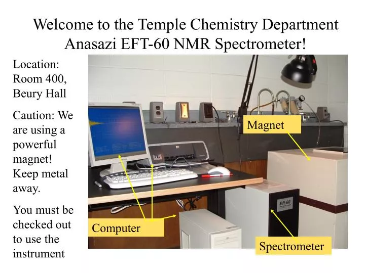
Welcome to the Temple Chemistry Department Anasazi EFT-60 NMR Spectrometer!. Location: Room 400, Beury Hall Caution: We are using a powerful magnet! Keep metal away. You must be checked out to use the instrument. Magnet. Computer. Spectrometer.

E N D
Welcome to the Temple Chemistry Department Anasazi EFT-60 NMR Spectrometer! Location: Room 400, Beury Hall Caution: We are using a powerful magnet! Keep metal away. You must be checked out to use the instrument Magnet Computer Spectrometer
This procedure will require you to use two different software applications The first is PNMR. This program runs the hardware and measures the spectrum. It saves the raw data to the disk. The second is NUTS. This is a data processing program. You will pass data made by the PNMR program to the NUTS program for processing and plotting. The programs are both running on the PC and you can use the menu bar to click back and forth between them.
Some Basics you need to know….. Prepare samples in a Deuterated solvent at ca. 10% w/v Solvent volume should be ca. 0.5 mL NMR tubes are fragile, precision cells. Handle carefully! Don’t drop the spinner collar! If dropped it will be damaged. Top of magnet, with cover opened A Properly filled NMR sample tube, 0.5 mL volume Spinner collar Sample positioning guage (hole toward front) (view from front of magnet)
A closer look into the magnet chamber… This lever starts and stops the spinning. Leave in the On position (shown) Air Control valves. Do not adjust on your own. Sample Ejection button Entry port for sample into probe (view from right-hand side of magnet)
Changing tubes, to analyze your sample. Here with cover open, we retrieve the sample already in the magnet Push and hold the sample ejection button; the sample in the chamber will rise up. Use other hand and pick up by top of cell.
It is important to push the tube carefully into the spinner collar Then use the positioning gauge (hole) at the front of the magnet to gently push the cell down to the proper level. This protects the delicate probe parts and your sample from smashing into each other
Using a tissue, wipe the outside of the sample tube. (getting chemicals, dirt, grease etc. into the probe can degrade the performance) • Avoid touching the bottom surfaces of the spinner collar. • Make sure that the spinner collar is in place. • Make sure that the spinner collar is positioned correctly. • Holding your sample by the upper part of the glass cell, let your tube gently fall into the probe opening. • Your sample will begin to spin inside the magnet. You can verify this by ejecting and observing the motion of the tube. Now close the plastic lid over the sample chamber. • If the sample does not lower, pull the spin control lever up, then push back down.
The computer controls the measurement. You will find it running a program called “PNMR” PNMR has a blue screen that shows raw data. Commands are typed into the text line (gray box at bottom of the blue screen) Now, take a seat in front of the computer workstation…..
The Data Acquisition Screen You must adjust the NMR for your sample. This is called “shimming” At the H1>prompt in the gray line, type: shim<ret> You will see a box in the screen asking for a time, type in 5, then click OK Command line for typing in commands
Now the Shimming Procedure takes over……. When finished, this gray box disappears. Your see a display like this one…
Starting your NMR measurement…… At the H1> prompt on the command line, type zg<ret> You will first get a file naming box, since the data will be written on the hard drive. Enter a filename, and click Save.
Data Collection Now your data collection begins. The result is displayed as a decaying curve. This is called a FID (or free induction decay) or interferogram. We can’t interpret data in this form, so it needs to be ported to another program and processed into a usable form. When the data collection is finished, mouse down to the task bar and click to the NUTS application
How do I take a 13C NMR? 13C NMR is a little more challenging, since the sensitivity compared to proton NMR is lower by a factor of 6000. We address this by: Using more compound, and using no more volume than needed (keeps concentration high) Taking more scans We load in the setup parameters for 13C at the prompt: >nu C13
How much more compound? About 100 mg of a organic compound of “normal” molecular weight. (say <200 da) can be done in one hour. About 25 mg of the same compound will require overnight data acquisition. In either case, use sample volume of 0.5mL. Neat liquids are OK, otherwise make up the volume so that 0.5 mL of the nmr tube is filled. (about 1” high)
After you get the C13> prompt, type “shim” (without quotes) The parameters automatically change back to 1H, and the trace on the screen automatically responds as the shimming is fixed. When the shimming is finished, the gray box in upper right-hand part of screen will disappear.
Next, take a “quick and dirty” 1H NMR by typing zgh at the >C13 prompt. When the scan is done, click into the NUTS window, and type a2. This will display your proton spectrum. You can check at this point to make sure the signals come at their proper shifts. In this spectrum, we see the water peak has drifted from its corrrect position. This needs to be fixed. Click back into the PNMR window.
Now if the shifts need to be rescaled…type zo at the prompt. Then in the second dialog box, enter the correct value… The z0 value on the screen will update. Type zgh again, then go to NUTS In the first gray window type the current (wrong) line position in ppm.
Now in NUTS, type a2. Your spectrum should be correctly positioned. You might want to “save” the proton spectrum at this point. The “Save As” dialog will allow you to direct the file to be saved to your own USB memory stick, mounted in the receptacle on the front of the computer. The new zo number now has water at its proper chemical shift. Now go back to the PNMR application
Taking a 13C spectrum First the program asks how you want to save the data file. The default is “PNMRFID”, but you should point the Save to your own, e.g., USB memory stick and make up a relevant name. At the C13> prompt, type zg As “zg” begins, the program will ask if you want to use “Broadband Decoupling” This is the preferred option, since it will make each the carbon signal into a single line. (If we don’t turn on the decoupling, the carbon signals will be split into multiplets from their hydrogen neighbors.) A box appears first, asking you to type 1 (BB decoupling) or 0 (no decoupling) Enter a 1 in the dialog box. Our 13C spectrum begins to acquire, by adding scans to the memory
Taking a large number of scans (for samples less than 50 mg) Set up the 13C parameters as on the earlier pages. However, instead of typing zg, type bapr at the C13> prompt. This runs a macro that will take a series of repetitive blocks of data, and store on the disk. In this example, we could type 10 into the box, and get 10 spectra, each consisting of 64 scans. We will use the NUTS software to add these together. We can’t just take 640 scans, because the instrument’s magnetic field drifts. Dialog boxes will also ask you to select: BB decoupling[1/0] And shimming between blocks [1/0] Yes to both questions Also, you must provide a file name to save blocks into.
Data Processing After switching over to the “NUTS” application, type at the > prompt: A2 (no enter needed) Your data will display on the screen as a spectrum.
Plotting out the Data, and Finishing Up At the > prompt in NUTS type >RU A “File Open” dialog appears and you select a macro called aii_H1_auto.mac, then click Open. Now click OK in the dialog box that follows Now your spectrum will print out, with the peak areas integrated, and peak positions listed on the printout. Click/pulldown: FILE|SaveAs and save your data in the folder on your own USB memory stick (jump drive). Use a short descriptive name, for future retrieval. Click Save,. File can be re-read and expanded etc, using NUTS in 2nd floor computer lab. As an alternative, you may (as your instructor may request) output the data for use with the JCAMP viewer software. To do this you must convert the file into JCAMP format, as shown, and save the converted file to your folder. Note, you must name the converted file with a .jdx or .dx extension or the viewer will not recognize it. Last, remove your sample as you did originally, and replace the reference sample into the spinner collar (has yellow “CDCl3” solvent blank label) You are finished, Congratulations!
If you chose the Block averaged method for 13C, the PNMR program has created a large number of “blocks” each of which has a spectrum stored on the disk. NUTS has to be told to handle this kind of data in a slightly different manner. directions…. While Block 1 is running in PNMR, switch to NUTS and type a2. Use the Zoom tool, and isolate on a single peak. Type the number 0. This sets a peak that, for all the other blocks will move a little to the right or left so they are all lined up, and then the adding of the blocks will work. When all the blocks have completed, in PNMR, switch to NUTS and type RU. From the macro list, choose aii_C13_bapr.mac | then, Open. Processing the Block-averaged data. Then choose the name of the file you saved the blocks into.
The data will appear as a single trace, the result of adding up several spectra. 80 blocks of 64 scans each You won’t see this stack of noisy spectra..