Random Walks and Semi-Supervised Learning
Random Walks and Semi-Supervised Learning. Based on : Xiaojin Zhu. Semi-Supervised Learning with Graphs. PhD thesis. CMU-LTI-05-192, May 2005

Random Walks and Semi-Supervised Learning
E N D
Presentation Transcript
Random Walks and Semi-Supervised Learning Based on : Xiaojin Zhu. Semi-Supervised Learning with Graphs. PhD thesis. CMU-LTI-05-192, May 2005 Page, Lawrence and Brin, Sergey and Motwani, Rajeev and Winograd, Terr.yThe PageRank Citation Ranking: Bringing Order to the Web. Technical Report. Stanford InfoLab, 1999. Ya Xu. SEMI-SUPERVISED LEARNING ON GRAPHS– A STATISTICAL APPROACH. PhD Thesis, STANFORD UNIVERSITY, May 2010 Longin Jan Latecki
Random walk propagates information on a graphbased on similarity of graph nodes Graph of web pages Graphs of hand written digits
Structure of real graphs One of the most essential characteristics is sparsity. The total number of edges in real graphs, particularly in large real graphs, usually grows linearly with the number of nodes n (instead of n2 as in a fully connected graph). As we can see in the table in all four real graphs the average degrees are less than ten, even though there are thousands of nodes. The sparsity property makes it possible to scale many prediction algorithms to very large graphs. Another key property is the degree distribution, which gives the probability that a randomly picked node has a certain degree. It follow a power-law distribution, which means there is usually only a very small fraction of nodes that have very large degrees.
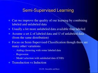
Semi-Supervised Learning • Large amounts of unlabeled training data • Some limited amounts of labeled data
Graph Construction Example • Verteciesare objects • The edge weights are determined by shape similarity
Key idea of random walk label propagation • Pair-wise similarity lacks accuracy in some cases • The similarity propagated among objects is helpful for revealing the intrinsic relation. The two horses are very different so that the dog looks more similar to the left horse. However, their similarity is reviled in the context of other horses. Random walk allows us to find paths that link them.
Problem Setup {(x1, y1) . .. (xl, yl)} be the labeled data, y in {1 . . .C}, and {xl+1 . . . xl+u} the unlabeled data, usually l << u. Hence we have total of n = l + u data points. We will often use L and U to denote the sets of labeled and unlabeled data. We assume the number of classes C is known, and all classes are present in the labeled data. We study the transductive problem of finding the labels for U. The inductive problem of finding labels for points outside of L and U will not be discussed. Intuitively we want data points that are similar to have the same label. We create a graph where the nodes are all the data points, both labeled and unlabeled. The edge between nodes i, j represents their similarity. We assume the graph is fully connected with the following weights: where α is a bandwidth hyperparameter.
Label Propagation Algorithm We assume that we only have two label classes C = {0, 1}. YL is l × 1 label of ones. f is n × 1 vector of label probabilities, e.g., entry f(i) is the probability of yi=1. We want that f(i) = 1 if i belongs to L. The initialization of f for unlabeled points is not important. The label propagation algorithm: or equivalently:
Random Walk Interpretation Imagine a random walk on the graph. Starting from an unlabeled node i, we move to a node j with probability Pij after one step. The walk stops when we hit a labeled node. Then f(i) is the probability that the random walk, starting from node i, hits a labeled node with label 1. Here the labeled node is viewed as an absorbing state. This interpretation requires that the random walk is irreducible and aperiodic.
Random Walk Hitting Probability According to slide 30 in Markov Processweneed to solve: Since we know that fL is composed of ones for label points, we only need to find fU: The fact that the matrix inverse exists follows from the next slides.
For Label Propagation algorithm we want to solve: Since P is row normalized, and PUU is a sub-matrix of P, it follows: Hence 0 and we obtain a closed form solution:
The identity holds if and only if the maximum of the absolute values of the eigenvalues of A is smaller than 1. Since we assume that A has nonnegative entries, this maximum is smaller than or equal to the maximum of the row-wise sums of matrix A. Therefore, it is sufficient to show that the sum of each row of A is smaller than 1.
Energy Minimization Interpretation The solution f minimizes the following energy function over all functions under the constraint that f(i) = 1 if i belongs to L. This energy can be equivalently written as where is graph Laplacian and D is a diagonal matrix with The solution f also minimizes the following for large λ0, where Y(0) =YL:
More on Graph Laplacian Given is an undirected graph G=(V, E, W), where V is a set of n vertices, E is set of edges, and W is a symmetric n x n weight or (affinity) matrix with all nonnegative entries such that w(i,j) = 0 if and only if there is no edge between nodes i and j. We consider two different definitions of graph Laplacian :
Example of a Graph Laplacian Computer the Laplacian for the following graph:
Proof: a) (b) follows directly from (a). (c) is a trivial result of (a) and the following