Continuous Probability Distributions
This document provides a comprehensive overview of continuous probability distributions commonly encountered in statistics, including the Uniform, Normal, Gamma, and Exponential distributions. It illustrates key properties, such as mean and variance, along with practical applications and example calculations. Detailed explanations accompany the Normal distribution, known for its Gaussian bell shape, and its importance in statistical analysis. The document also explores the relationships between different distributions and their characteristics, crucial for interpreting data and conducting hypothesis tests.


Continuous Probability Distributions
E N D
Presentation Transcript
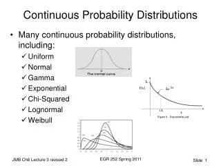
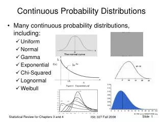
Continuous Probability Distributions • Many continuous probability distributions, including: • Uniform • Normal • Gamma • Exponential • Chi-Squared • Lognormal • Weibull EGR 252 Fall 2011
Uniform Distribution • Simplest – characterized by the interval endpoints, A and B. A ≤ x ≤ B = 0 elsewhere • Mean and variance: and EGR 252 Fall 2011
Example: Uniform Distribution A circuit board failure causes a shutdown of a computing system until a new board is delivered. The delivery time X is uniformly distributed between 1 and 5 days. What is the probability that it will take 2 or more days for the circuit board to be delivered? EGR 252 Fall 2011
Normal Distribution • The “bell-shaped curve” • Also called the Gaussian distribution • The most widely used distribution in statistical analysis • forms the basis for most of the parametric tests we’ll perform later in this course. • describes or approximates most phenomena in nature, industry, or research • Random variables (X) following this distribution are called normal random variables. • the parameters of the normal distribution are μand σ(sometimes μand σ2.) EGR 252 Fall 2011
(μ = 5, σ = 1.5) Normal Distribution • The density function of the normal random variable X, with mean μ and variance σ2, is all x. EGR 252 Fall 2011
Standard Normal RV … • Note: the probability of X taking on any value between x1 and x2 is given by: • To ease calculations, we define a normal random variable where Z is normally distributed with μ = 0 and σ2= 1 EGR 252 Fall 2011
Standard Normal Distribution • Table A.3 Pages 735-736: “Areas under the Normal Curve” EGR 252 Fall 2011
Examples • P(Z ≤ 1) = • P(Z ≥ -1) = • P(-0.45 ≤ Z ≤ 0.36) = EGR 252 Fall 2011
Name:________________________ • Use Table A.3 to determine (draw the picture!) 1. P(Z≤ 0.8) = 2. P(Z≥ 1.96) = 3. P(-0.25 ≤ Z≤ 0.15) = 4. P(Z ≤ -2.0 orZ≥ 2.0) = EGR 252 Fall 2011
Applications of the Normal Distribution • A certain machine makes electrical resistors having a mean resistance of 40 ohms and a standard deviation of 2 ohms. What percentage of the resistors will have a resistance less than 44 ohms? • Solution: Xis normally distributed with μ = 40 and σ= 2 and x = 44 P(X<44) = P(Z< +2.0) = 0.9772 Therefore, we conclude that 97.72% will have a resistance less than 44 ohms. What percentage will have a resistance greater than 44 ohms? EGR 252 Fall 2011
The Normal Distribution “In Reverse” • Example: Given a normal distribution with μ = 40 and σ = 6, find the value of X for which 45% of the area under the normal curve is to the left of X. Step 1 If P(Z < z) = 0.45, z = _______ (from Table A.3) Why is z negative? Step 2 X = _________ 45% EGR 252 Fall 2011
Normal Approximation to the Binomial • If n is large and p is not close to 0 or 1, or if n is smaller but p is close to 0.5, then the binomial distribution can be approximated by the normal distribution using the transformation: • NOTE: add or subtract 0.5 from X to be sure the value of interest is included (draw a picture to know which) • Look at example 6.15, pg. 191 (8th edition) EGR 252 Fall 2011
Look at example 6.15, pg. 191-192 p = 0.4 n = 100 μ= ____________ σ= ______________ if x = 30, then z = _____________________ and, P(X < 30) = P (Z < _________) = _________ EGR 252 Fall 2011
Your Turn DRAW THE PICTURE!! • Refer to the previous example, • What is the probability that more than 50 survive? • What is the probability that exactly 45 survive? EGR 252 Fall 2011
Gamma & Exponential Distributions • Related to the Poisson Process (discrete) • Number of occurrences in a given interval or region • “Memoryless” process • Sometimes we’re interested in the number of events that occur in an area (eg flaws in a square yard of cotton). • Sometimes we’re interested in the time until a certain number of events occur. • Area and time are variables that are measured. • Typical problem statement: The length of time in days between student complaints about too much homework follows a gamma distribution with α = 3 and β = 7. What is the probability that up to two weeks will elapse before 6 complaints are heard? EGR 252 Fall 2011
Gamma Distribution • The density function of the random variable X with gamma distribution having parameters α (number of occurrences) and β (time or region). x > 0. μ = αβ σ2= αβ2 EGR 252 Fall 2011
Exponential Distribution • Special case of the gamma distribution with α = 1. x > 0. • Describes the time until or time between Poisson events. μ = β σ2= β2 EGR 252 Fall 2011
Is It a Poisson Process? • For homework and exams in the introductory statistics course, you will be told that the process is Poisson. • An average of 2.7 service calls per minute are received at a particular maintenance center. The calls correspond to a Poisson process. What is the probability that up to a minute will elapse before 2 calls arrive? • An average of 3.5 service calls per minute are received at a particular maintenance center. The calls correspond to a Poisson process How long before the next call? EGR 252 Fall 2011
Poisson Example Problem An average of 2.7 service calls per minute are received at a particular maintenance center. The calls correspond to a Poisson process. What is the probability that up to 1 minute will elapse before 2 calls arrive? • β = 1 / λ = 1 / 2.7 = 0.3704 • α = 2 What is the value of P(X ≤ 1) Can we use a table? No We must use integration. EGR 252 Fall 2011
Poisson Example Solution An average of 2.7 service calls per minute are received at a particular maintenance center. The calls correspond to a Poisson process. What is the probability that up to 1 minute will elapse before 2 calls arrive? β = 1/ 2.7 = 0.3704 α = 2 P(X < 1) = (1/ β2) x e-x/ β dx = 2.72 x e -2.7x dx = [-2.7xe-2.7x – e-2.7x] 01 = 1 – e-2.7 (1 + 2.7) = 0.7513 EGR 252 Fall 2011
Another Type of Question An average of 2.7 service calls per minute are received at a particular maintenance center. The calls correspond to a Poisson process. What is the expected time before the next call arrives? Expected value = μ= αβα = 1 β = 1/2.7 μ = β = 0.3407 min. We expect the next call to arrive in 0.3407 minutes. When α = 1 the gamma distribution is known as the exponential distribution. EGR 252 Fall 2011