Download
1 / 16
160 likes | 175 Views
Investigating universe creation and dynamics with simplifying rules and quantum gravity concepts. Correlating temperature fluctuations to boundary correlations in a theoretical framework.

E N D
KEK-WS 03/14/2007 Evolution of Simplicial Universe Shinichi HORATA and Tetsuyuki YUKAWA Hayama center for Advanced Studies, Sokendai Hayama, Miura, Kanagawa 240-0193, Japan Some of the topics have been already appeared in S.Horata, and T.Yukawa : Making a Universe.hep-th/0611076. e-mail address: yukawa@soken.ac.jp
Motivated by the Observation of CMB anisotropies WMAP (Wilkinson Microwave Anisotropy Probe) 2003 COBE (Cosmic Background Explorer) 1996 (2006 Nobel Prize) Temperature fluctuation T~2.7K
Phenomenological Problem : Obtain the two point correlation function of temperaturefluctuations in the CMB Correlation beyond the event horizon Fundamental Problems : How has the universe started ? Initial condition How has it evolved ? Cosmological dynamics What is the space-time of the universe? Direction and expanse How did the physical laws appear ? Physical reality Creation by rules, without laws
A simplest example of the creation without laws : The Peano axioms (rules) for the natural number 1. Existence of the element ‘1’. 2. Existence of the successor ‘S (a )’ of a natural number ‘a’. Axioms for creating the universe. 1. Existence of the element ‘d-simplex’. 2. Existence of the neighbors of simplicial complex. For example, creating a 2-dimensional universe 1. The element =anequilateral triangle 2. The neighbor =2-d triangulated surfaces constructed under themanifold conditions: • Two triangles can attach • through one link (face). ii) Triangles sharing one vertex form a disk (or a semi-disk).
Simplicial Quantum Gravity Appendix 1. Space Quantization = Collection of all the possible triangulated (simplicial) manifolds dimple phase Phase transition Simplicial S2 manifold S.Horata,T.Y.(2002) K-J.Hamada(2000)
Quantum Universe: Collection of all possible d-simplicial manifold Extension to open topology Example S2 to D3 {DV,DS }movesof D3 topology (p,q) moves of S2 topology {1,2} (1,3) (1,3) (3,1) {1,0} (2,2) (2,2) {1,-2} (3,1)
Evolution of the 2d quantum universe in computer Start with an elementary triangle, and create a Markov chain by selecting moves randomly under the condition ofdetailed balance. pa: a priori probability weight for a configuration a, na: number of possible moves starting from a configuration a (global and additive) with the volumeV= and the areaS= a m :the (lattice) cosmological constant mB :the (lattice) boundary cosmological constant
Simplest universes at the early stage N2 A universe withN2=19,N~1=18 a lot of trees and bushes -> Tutte algorithm
Appendix2. (Old ) Matrix Model Generating function k: # of triangles, l: # of boundary links BIPZ(1978) Conjecture from the singularity analysis diverges at continuous limit
3 Phases of the 2-dimensional universe <N2> Im[Z(g,j)] < >
Defining the Physical timet with a dimensional factor cby t S(t) V(t) Monte Carlo timet and physical timet are related as N.B. t becomes negative when the volume decreases. In the expanding phase computer simulation shows,V~V0 t, S~S0 t,thus we have ( on ) matrix model which means theinflation in t:
Appendix 3. The Liouville theory Liouville action with a boundary Q: background charge (=b+b-1) l: thecosmological constant lB: theboundary cosmological constant Partition function Fateev,A.&Al.Zamolodchikovhep-th0001012 b2=2/3 for pure gravity
In the classical limit Classical Liouville equation for the expanding region Homogeneous solution (f0=const. ) Physical timet and the conformal timeh Line element expands as Inflation N.B. Our definition of the physical time coincide with this physical time.
Identifyingthe distance The boundary two point correlation function Conformal theory predicts quantum+ ensemble averages The boundary metric densityexp{bf (x)} ~thenumber of triangles shearing a boundary vertex x+n-th neighbors x + 1st neighbors Geodesic distanceD = Smallest number of links connecting two vertices x ~geodesic distanceD
Evolution of the correlation function Boundary 2-point function Measured on one universe. Angular power spectra L(t) =boundary length att Large angle correlation
Future Problems : • Extension to the 4-dimension • Inclusion of Matter • Creation of Dynamical Laws (preliminary) The power spectrum of the 2-point correlation function on a last scattering surface lss (S2) in S3 of D4 N.B. Normalized atl=10