Download
1 / 8
80 likes | 193 Views
Hydrology Virtual Mission for WATERHM. Doug Alsdorf, Ohio State U. Mike Durand, Jim Hamski, Brian Kiel, Gina LeFavour, Jon Partsch Dennis Lettenmaier, U. Washington Kostas Andreadis, Liz Clark Delwyn Moller, JPL. What is the VM?.

E N D
Hydrology Virtual Mission for WATERHM • Doug Alsdorf, Ohio State U. • Mike Durand, Jim Hamski, Brian Kiel, Gina LeFavour, Jon Partsch • Dennis Lettenmaier, U. Washington • Kostas Andreadis, Liz Clark • Delwyn Moller, JPL
What is the VM? • Goal: to define the spatial and temporal trade-offs when measuring storage changes and discharge. • Goal accomplished by answering 3 key questions: • What are the spatial and temporal samplings of ΔS and Q required to accurately constrain weather and climate models? • Storage change plays a hydrologic role in many basins, but is knowing ΔS sufficient, or is Q also required to accurately constrain the water balance? • Can reach-to-reach discharge variations be accurately measured from space?
How will the VM work? • We will conduct the following tasks to address the 3 questions: • Various orbital tracks will be overlaid on a global VIC model-based mapping of ΔS and Q to determine the percentages of ΔS and Q that can potentially be sampled. Rather than only knowing the percentages of water bodies missed, this will demonstrate the percentages of ΔS and Q measured for each basin’s water balance as dictated by various orbits and sampling technologies. • VM-I creates model h surfaces with errors expected from a spaceborne technology. These simulated h values will be used to construct storage changes in three selected basins, and resulting ΔS values will be compared to VIC model supplied Q values (and Q values from Task 3). • Our initial SRTM-based Manning’s-method of estimating Amazon discharge will be expanded to other rivers and channel cross-sectional geometries will be investigated for constraining Q. An alternative method of estimating discharge will be constructed in a data assimilation of instrument simulated h surfaces (i.e., from Task 2 above). Spatial and temporal sampling resolutions and errors will be investigated in both Q methods. • The instrument simulator of VM-I will be enhanced (and applied in the Tasks 2 and 3) with layover identification, assessment of height accuracies as bounded by the use of the SRTM DEM for instrument calibration, and quantification of h averaging schemes.
( ) Q2 ¶ ¶ z ¶ Q g + + ¶ t ¶ x A ¶ t 1 1 zw A A 2/3 ( ) zw n 2z+w ¶ Q ¶ h q - w = ( ) 1/2 ¶ x ¶ t ¶ h ¶ x The VM Concept Simple Moderate Q = z = (h-bathymetry) • The VM uses both model and real data, and uses complex and simple techniques. Complex = g(S0-Sf) S0 = bathymetric slope Sf = friction or energy slope, i.e., dh/dx Synthetic World Real World VIC LISFLOOD Instrument Simulator SRTM Altimetry InSAR Imagery • Use data assimilation to introduce “errors” (P, Z) and varying sampling resolutions to determine their impacts on estimating Q and measuring S. • Use Manning’s n approach to estimate Q and measure S. • Use DA to estimate Q • Manning’s equation, Continuity to estimate Q These are designed to assess Q from existing satellite measurements. Key: all parameters can be measured from space, but not depth (n is empirical).
We can measure width • Uses classification based on 30m Landsat data 69 meters Pavelsky & Smith, algorithm in review
What does SRTM tell us? • SRTM h accuracy is too coarse for reaches < 100s kms, but Q is not too bad! Q m3/s Observed SRTM Error Tupe 63100 62900 -0.3% Itapeua 74200 79800 7.6% Manacapuru 90500 84900 -6.2%
What does repeat-pass InSAR tell us? • Floodplains have complex patterns of water flow, use continuity to get flux
First Results from Data Assimilation • See next presentation on Ohio River data assimilation • Preliminary feasibility test shows successful estimation of discharge by assimilating satellite water surface elevations • Nominal 8 day overpass frequency gives best results; effect of updating largely lost by ~ 16 days • Results are exploratory and cannot be assumed to be general -- additional experiments with more realistic hydrodynamic model errors (Manning’s coefficient, channel width etc), hydrologic model errors, and more topographically complex basins (e.g. Amazon River) are needed. • Assumption that “truth” and filter models (both hydrologic and hydrodynamic) are identical needs to be investigated