Download
1 / 38
380 likes | 547 Views
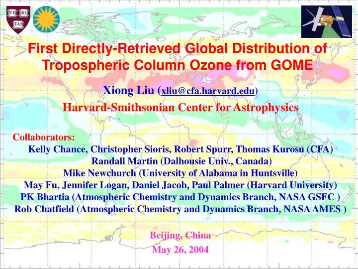
First Directly-Retrieved Global Distribution of Tropospheric Column Ozone from GOME. Xiong Liu ( xliu@cfa.harvard.edu ) Harvard-Smithsonian Center for Astrophysics Collaborators: Kelly Chance, Christopher Sioris, Robert Spurr, Thomas Kurosu (CFA) Randall Martin (Dalhousie Univ., Canada)

E N D
First Directly-Retrieved Global Distribution of Tropospheric Column Ozone from GOME Xiong Liu (xliu@cfa.harvard.edu) Harvard-Smithsonian Center for Astrophysics Collaborators: Kelly Chance, Christopher Sioris, Robert Spurr, Thomas Kurosu (CFA) Randall Martin (Dalhousie Univ., Canada) Mike Newchurch (University of Alabama in Huntsville) May Fu, Jennifer Logan, Daniel Jacob, Paul Palmer (Harvard University) PK Bhartia (Atmospheric Chemistry and Dynamics Branch, NASA GSFC ) Rob Chatfield (Atmospheric Chemistry and Dynamics Branch, NASA AMES ) Beijing, China May 26, 2004
Outline • Introduction to Ozone and Tropospheric Ozone • Satellite-based Tropospheric Ozone Retrievals • Algorithm Description • Intercomparison with TOMS, Dobson, and Ozonesonde observations • Examples of Daily Retrievals • Global distribution of Tropospheric Column Ozone and comparison with the 3D GEOS-CHEM model • Summary and Future work • Atmospheric Measurements and Studies at Harvard-Smithsonian CFA (Time allowed)
Stratopause Ozone layer Tropopause Ozone • First discovered by Schönbein [1840], a reactive oxidant in the atmosphere. • First quantitative observation: early 20th century in Europe (e.g., Dobson, Götz) • First discovery of ozone hole by Farman et al. [1985] • First attempts to understand ozone in the 1930s. Until the last 30-40 years, the stratospheric ozone chemistry (NOx, HOx, ClOx) is well understood. • Noble chemistry prizes were awarded to Paul Crutzen, Mario Molina, and Sherwood Rowland in 1995. Courtesy of Randall Martin
OH HNO3 NO2 NOx O3 OH HOx HO2 H2O2 hv, H2O CO, VOCs CO, VOCs, NOx Tropospheric Ozone • Key species in climate, air quality, and tropospheric chemistry • Major Greenhouse gas, 15-20% of climate radiative forcing • Primary constituents of photochemical smog • Largely controls tropospheric oxidizing capacity Simplified Tropospheric O3 Chemistry NO Courtesy of Randall Martin
Residual-based Satellite Tropospheric Ozone Retrievals • Why satellite observations: global coverage • Challenge: only 10% of Total column Ozone (TO) • Residual-based approaches: TO – Strat. Column Ozone(SCO) • Tropospheric ozone residual: TOMS minus SAGE/SBUV/HALOE/MLS [Fishman et al., 1990, 2003, Ziemke et al., 1998, Chandra et al., 2003] • Cloud/clear difference techniques: [Ziemke et al., 1998; Newchurch et al., 2003, Valks et al., 2003] • Modified residual method [Kim et al., 1996; Hudson et al., 1998] • Topographic contrast method [Jiang et al., 1996, Kim and Newchurch et al., 1996, Newchurch et al., 2003] • Scan-angle method (Special) [Kim et al., 2001] • Limits: poor spatiotemporal resolution and large spatiotemporal variability of SCO mostly climatological or tropics • Limb/Nadir matching: TO/SCO from same instrument or satellite
ESAGlobal Ozone Monitoring Experiment • Launched April 1995 on ERS-2 • Nadir-viewing UV/vis/NIR • 240-400 nm @ 0.2 nm • 400-790 nm @ 0.4 nm • Footprint 320 x 40 km2 • 10:30 am cross-equator time • Global coverage in 3 days
GOME Radiance Spectrum and Trace Gases Absorption Atmospheric trace gas absorptions detected in satellite spectra
Physical Principles of Ozone Profile Retrieval (UV/Vis.) Hartley & Huggins bands (245-355 nm) Huggins bands (318-340 nm) • Wavelength-dependent O3 absorption & dependence of Rayleigh scattering provide discrimination of O3 at different altitudes from backscattered measurements. • Temperature-dependent ozone absorption in the Huggins bands provides additional tropospheric ozone information. Chappuis bands (400-800 nm) Chance et al., 1997
Ozone Profile Retrieval from GOME • Direct tropospheric ozone retrieval: daily global distribution of tropospheric ozone without other SCO measurements or deriving SCO • Several groups [Munro et al., 1998; Hoogen et al., 1999; Hasekamp et al., 2001; van der A et al, 2002; Muller et al., 2003] have developed ozone profile retrieval algorithms from GOME: each of them demonstrates that limited tropospheric ozone information can be detected. • However, global distribution of tropospheric column ozone has not been published from these algorithms • Require accurate and consistent calibrations. • Need to fit the Huggins bands to high precision. • Tropospheric column ozone is only ~10% of total column ozone • Limited Vertical Resolution
Algorithm Description • Ill-posed problem: non-linear optimal estimation [Rodgers, 2000] Y: Measurement vector (e.g., radiances) • X, Xi, Xi+1: State vector (e.g. ozone profile) • Xa: a priori state vector • K : Weighting function matrix, sensitivity of radiances to ozone • Sa: A priori covariance matrix • Sy: Measurement error covariance matrix
IB,c IB,o Rc Ro Pc dt Rs Algorithm Description — Radiative Transfer Simulation • Radiative transfer model: LIDORT [Spurr et al., 2001] • Model Ring effect with a first-order single-scattering model • Radiance polarization correction with a look-up table • Forward model inputs • SAGE strat. [Bauman et al., 2003] & GOCART trop. aerosols [Chin et al., 2002] • Daily ECMWF T profiles and NCEP Ps • Clouds: Lambertian surfaces • Cloud-top pressure from GOMECAT [Kurosu et al., 1999] • Cloud fraction derived at 370.2 nm with surface albedo database [Kolemeijer et al.,2003] • Wavelength dependent albedo (2-order polynomial) from 326-339 nm to take account of residual aerosol and cloud effects
AlgorithmDescription • Perform external wavelength and radiometric calibrations • Derive variable slit widths and shifts between radiances/irradiances • Co-add adjacent pixels from 289-307 nm to reduce noise • Perform undersampling correction with a high-resolution solar reference • Fit degradation for 289-307 nm on line in the retrieval • Optimize fitting windows: 289-307 nm, 326-339 nm • Latitude/monthly dependent TOMS V8 climatology • Retrieval Grid: 11 layers, use daily NCEP tropopause to divide the troposphere and stratosphere, 2-3 tropospheric layers • Tropospheric column ozone: sums of tropospheric partial columns • State Vector: 47 variables (ozone, Ring, surface albedo, undersampling, degradation, wavelength shifts, NO2, SO2, BrO) • Spatial resolution: 960×80 km2
Averaging Kernels (DX’/X) 8-12 km (at 20-38 km) VR: 7-12 km (at 10-37 km) 7-12 km (at 7-37 km)
A Priori Influence A Priori influence in TCO: 15% in the tropics, 50% at high-latitudes
Retrieval Errors Precision Smoothing TO: <2 DU(0.5); 3 DU (1.0%) SCO: <2 DU(1%); 2-5 DU (1-2%) TCO: 1.5-3 DU(6-12%); 3-6 DU(12-25%) Precision: 2-8% (< 2DU) in the strat., <12%(5DU) in the troposphere Smoothing: 10% at 20-40 km, 15% at > 40 km, and 30% at <10 km
An Orbit of Retrieved Ozone Profiles Ozone Hole (120 DU) Biomass burning
Validation • GOME data are collocated at 33 WOUDC ozonesonde stations during 96-99. • Validate retrievals against TOMS V8, Dobson/Brewer total ozone, and ozonesonde TCO. • Data mostly from WOUDC • Collocation criteria: • Within ~8 hours, 1.5° latitude and ~500 km in longitude • Average all TOMS points within GOME footprint • Number of comparisons: 4711, 1871, and 1989 with TOMS, Dobson, and ozonesonde, respectively. Circles: with Dobson/Brewer TO http://www.woudc.org http://croc.gsfc.nasa.giv/shadoz http://toms.gsfc.nasa.gov http://www.cmdl.noaa.gov
Total Column Ozone Comparison • GOME-TOMS/Dobson: within retrieval uncertainties and saptiotemporal variability. • Means Biases: <6 DU (2%) at most stations • 1: 2-4 DU (1.5%) in the tropics, <6.1 DU (2.4%) at higher latitudes • Means Biases: <5 DU (2%) at most stations • 1: 3-6 DU (<3%) in the tropics, <8-16 DU (<5%) at higher latitudes TOMS DOBSON A PrioriRetrieval DobsonTOMS
GOME-SONDE within retrieval uncertainties. • Biases: <4 DU(15%) except –5.5, 4.4, 5.6DU(16-33%) at NyÅlesund, Naha, Tahiti • 1 : 3-7 DU(13-28%) • Capture most of the temporal variability • GOME-SONDE within retrieval uncertainties. • Biases: <3.3 DU(15%) • 1 : 3-8 DU(12-27%) A PrioriRetrieval Ozonesonde A PrioriRetrieval Ozonesonde Tropospheric Column Ozone Comparison
GEOS-CHEM global 3D tropospheric chemistry and transport model • Driven by NSAA GEOS-STRAT GMAO met data [Bey et al., 2001] • 22.5o resolution/26 vertical levels • O3-NOx-VOC chemistry • Recent anthropogenic, biogenic, natural emissions • Synoz flux: 475 Tg O3 yr-1 from stratosphere • A 18-month simulation (June 1996-Nov 1997)
Examples of Daily Retrievals 97-98 El Nino Event Java [110-125E, 6.6-8.6S] America Samoa [180-158E, 13.2-15.2S]
Examples of 3-Day Composite Global Maps Biomass burning LOW TCO over the Pacific Mid-latitudes High TCO Band High-latitude high TCO Transport of mid-latitude high TCO air to the tropics
GOME vs. GEOS-CHEM • Similar overall structures • Global biases: <2±4 DU, r=0.82-0.9 • SH: <1±2 DU,r=0.94-0.98 • NH: <4.3±4.6 DU, r=0.6-0.8
GOME vs. GEOS-CHEM • Usually within 5 DU. • Large positive bias of 5-15 DU at some northern tropical and subtropical regions: central America, tropical North Africa, Southeast Asia, Middle East • Usually >0.6. • Poor correlation: central America, equatorial remote Pacific, tropical North Africa and Atlantic, North high latitudes
GOME/GEOS-CHEM vs. MOZAIC (Central America) 50 40 30 20 • MOZAIC: www.aero.obs-mip.fr/mozaic • Data: 1994-2004 (vary from location to location) • Evaluate GOME/GEOS-CHEM TCO in seasonality
GOME/GEOS-CHEM vs. MOZAIC (Southeast Asia) A PrioriRetrieval GOES-CHEMMOZAIC
GOME/GEOS-CHEM vs. MOZAIC (Accra) A PrioriRetrieval GOES-CHEMMOZAIC
GOME/GEOS-CHEM vs. MOZAIC (Middle East) A PrioriRetrieval GOES-CHEMMOZAIC
Summary • Ozone profiles and Tropospheric Column Ozone (TCO) are retrieved from GOME using the optimal estimation approach. • Retrieved TO and TCO compare very well with TOMS, Dobson/Brewer, and ozonesonde measurements. • The retrievals clearly show signals due to convection, biomass burning, stratospheric influence, pollution, and transport, and are capable of capturing the spatiotemporal evolution of TCO in response to regional or short time-scale events. • The overall structures between GOME and GEOS-CHEM are similar, but some significant positive biases occur at some northern tropical and subtropical regions. • The GOME retrievals usually agree well with the MOZOAIC measurements, to within the monthly variability and some biases can be explained by the reduced sensitivity to lower tropospheric ozone, spatiotemporal variation, and the large spatial resolution of GOME retrievals.
Future Work • Improve retrieval algorithms (Chappuis bands, external degradation correction) and complete more than 8-year GOME data record. • Apply the algorithm to SCIMACHY, OMI, GOME-2, OMPS, or future geostationary satellite measurements. • Integrate with the GEOS-CHEM model and other in-situ data, improve our understanding of global/regional budget of tropospheric ozone • Tropospheric ozone radiative forcing Acknowledgements • This study is supported by the NASA and by the Smithsonian Institution. • Thank all collaborators. • We thank WOUDC and its data providers (e.g., SHADOZ, CMDL), TOMS, MOZAIC for providing correlative measurements. • We are grateful to NCEP/NCAR ECMWF reanalysis projects. • We appreciate the ongoing cooperation of the European Space Agency and the Germany Aerospace Center in the GOME program.
Comparison with SAGE-II (>15 km) • Comparison with SAGE-II V6.2 ozone profiles above 15 km during 1996-1997 (5732) • Means Biases: <15% • 1: <10% for the top seven layers and <15% for the bottom layer • Systematic biases in the retrievals but not in the a priori, suggesting residual measurement errors in the GOME level-1 data
A Priori Influence (06/7-9/1997) TOMS V8 A Priori Retrieval with TOMS V8 A Priori GEOS-CHEM A Priori Retrieval with GEOS-CHEM A Priori