Download
1 / 48
490 likes | 620 Views
Introduction to Seasonal Climate Prediction Liqiang Sun International Research Institute for Climate and Society (IRI). Weather forecast – Initial Condition problem Climate forecast – Primarily boundary forcing problem. Climate Forecasts. be probabilistic ensembling

E N D
Introduction to SeasonalClimate PredictionLiqiang SunInternational Research Institute for Climate and Society (IRI)
Weather forecast – Initial Condition problem Climate forecast – Primarily boundary forcing problem
Climate Forecasts • be probabilistic • ensembling • be reliable and skillful • calibration and verification • address relevant scales and quantities • downscaling
OUTLINE • Fundamentals of probabilistic forecasts • Identifying and correcting model errors • systematic errors • Random errors • Conditional errors • Forecast verification • Summary
Basis of Seasonal Climate Prediction Changes in boundary conditions, such as SST and land surface characteristics, can influence the characteristicsof weather(e.g. strength or persistence/absence), and thus influence the seasonal climate.
IRI DYNAMICAL CLIMATE FORECAST SYSTEM 2-tiered OCEAN ATMOSPHERE GLOBAL ATMOSPHERIC MODELS ECPC(Scripps) ECHAM4.5(MPI) CCM3.6(NCAR) NCEP(MRF9) NSIPP(NASA) COLA2 GFDL PERSISTED GLOBAL SST ANOMALY Persisted SST Ensembles 3 Mo. lead 10 POST PROCESSING MULTIMODEL ENSEMBLING 24 24 10 FORECAST SST TROP. PACIFIC (multi-models, dynamical and statistical) TROP. ATL, INDIAN (statistical) EXTRATROPICAL (damped persistence) 12 Forecast SST Ensembles 3/6 Mo. lead 24 24 30 12 30 REGIONAL MODELS 30
Contingency tables for 3 subregions of Ceara State at local scales (FMA 1971-2000) Contingency tables for 3 subregions of Ceara State at local scales (FMA 1971-2000) Contingency tables for 3 subregions of Ceara State at local scales (FMA 1971-2000) RSM RSM RSM RSM RSM RSM RSM RSM RSM OBS OBS OBS B B B Coast Coast Coast B B B N N N A A A 5 5 5 3 3 3 2 2 2 N N N 3 3 3 4 4 4 3 3 3 A A A 2 2 2 3 3 3 5 5 5 Probability Calculated Using the Ensemble Mean Contingency Table
Contingency tables for 3 subregions of Ceara State at local scales (FMA 1971-2000) Contingency tables for 3 subregions of Ceara State at local scales (FMA 1971-2000) Contingency tables for 3 subregions of Ceara State at local scales (FMA 1971-2000) RSM RSM RSM RSM RSM RSM RSM RSM RSM OBS OBS OBS B B B Coast Coast Coast B B B N N N A A A 5 5 5 3 3 3 2 2 2 N N N 3 3 3 4 4 4 3 3 3 A A A 2 2 2 3 3 3 5 5 5 Probability obtained from ensemble spread • Count the # of ensembles in each category, e.g., Total 100 Ensembles, • 40 ensembles in Category “A” • 35 ensembles in Category “N”, and • 25 ensembles in Category “B”. • 2) Calibration
Example of seasonal rainfall forecast (3-month average & Probabilistic)
Why seasonal averages? Rainfall correlation skill: ECHAM4.5 vs CRU Observations (1951-95) Should we onlybe forecasting for February for SW US & N Mexico?
Why seasonal averages? Partial Correlation Maps for Individual Months No independentskill for individualmonths.
Model Forecast (SON 2004), Made Aug 2004 RUN #1 RUN #4 Two ensemble membersfrom same AGCM, same SST forcing, justdifferent initial conditions. Why probabilistic? Observed Rainfall (SON 2004) Units are mm/season
Why probabilistic? Model Forecast (SON 2004), Made Aug 2004 1 5 2 6 Observed RainfallSep-Oct-Nov 2004(CAMS-OPI) 3 7 Seasonal climate is a combinationof boundary-forced SIGNAL, and chaotic NOISE from internaldynamics of the atmosphere. 4 8
Why probabilistic? Model Forecast (SON 2004), Made Aug 2004 ENSEMBLE MEAN Observed RainfallSep-Oct-Nov 2004(CAMS-OPI) Average model response, or SIGNAL, due to prescribed SSTswas for normal to below-normal rainfall over southern US/northern Mexico in this season. Need to also communicate fact that some of the ensemblemember predictions were actually wet in this region. Thus, there may be a ‘most likely outcome’, but there arealso a ‘range of possibilities’ that must be quantified.
Climate Forecast: Signal + Uncertainty “SIGNAL” Near-Normal “NOISE” BelowNormal AboveNormal Historical distribution Forecast distribution Forecast Mean Climatological Average The SIGNAL represents the ‘most likely’ outcome. The NOISE represents internal atmospheric chaos, uncertainties in the boundary conditions, and random errors in the models.
Probabilistic Forecasts Reliability: Forecasts should “mean what they say”. Resolution: Probabilities should differ from climatology as much as possible, when appropriate Reliability Diagrams Showing consistency between the a priori stated probabilities of an event and the a posteriori observed relative frequencies of this event.Good reliability is indicated by a 45° diagonal.
Optimizing Probabilistic Information • Eliminate the ‘bad’ uncertainty -- Reduce systematic errors e.g. MOS correction, calibration • Reliably estimate the ‘good’ uncertainty -- Reduce probability sampling errors e.g. Gaussian fitting and Generalized Linear Model (GLM) -- Minimize the random errors e.g. multi-model approach (for both response & forcing) -- Minimize the conditional errors e.g. Conditional Exceedance Probabilities (CEPs)
Systematic error in locationof mean rainfall, leads tospatial error in interannualrainfall variability, and thusa resulting lack of skilllocally. Systematic Spatial Errors
… as well as in the magnitude of its interannual variability. ORIGINAL Statistical recalibration of the model’sclimate and its response characteristicscan improve model reliability. RECALIBRATED Systematic Calibration Errors ORIGINAL RESCALED Dynamical models may have quantitativeerrors in the mean climate
Reducing Systematic ErrorsMOS Correction DJFM rainfall anomaly correlation before and after statistical correction UNAM (Tippett et al., 2003, Int. J. Climatol.)
N=8 N=16 N=39 N=24 Converges like S = Signal-to-noise ratio N = ensemble size “True” rms divide by .
Fitting with a Gaussian Two types of error: • PDF not really Gaussian! • Sampling error • Fit only mean • Fit mean and variance Error(Gaussian fit N=24) = Error(Counting N=40)
Minimizing Random ErrorsMulti-model ensembling Combining models reduces deficiencies of individual models Probabilistic skill scores (RPSS for 2m Temperature (JFM 1950-1995)
A Major Goal of Probabilistic Forecasts Reliability! Reliability Diagrams Showing consistency between the a priori stated probabilities of an event and the a posteriori observed relative frequencies of this event.Good reliability is indicated by a 45° diagonal.
Benefit of Increasing Number of AGCMs in Multi-Model Combination JAS Temperature JAS Precipitation (Robertson et al. 2004)
Conditional Exceedance Probabilities The probability that the observation exceeds the amount forecast depends upon the skill of the model. If the model were perfect, this probability would be constant. If it is imperfect, it will depend on the ensemble member’s value. Identify whether the exceedance probability is conditional upon the value indicated. Generalized linear models with binomial errors can be used, e.g.: Tests can be performed on 1 to identify conditional biases. If 1 = 0 then the system is reliable. 0 can indicate unconditional bias. (Mason et al. 2007, Mon Wea Rev)
Idealized CEPs Positive skillSIGNAL too weak PERFECT Reliability β1>0 β1=0 Positive skillSIGNAL too strong Negative skill NO skill β1<0|β1|>|Clim| β1<0 β1= Clim. (from Mason et al. 2007, Mon Wea Rev)
Standardized anomaly Scale Shift 100% 50% 0% Conditional Exceedance Probabilities (CEPs) Use CEPs to determinebiased probability ofexceedance. Shift model-predicted PDF towards goal of 50% exceedance probability. Note that scale is a parameter determined in minimizing the model-CEP slope.
CEP Recalibrationcan eitherstrengthen orweaken SIGNAL Adjustment decreases signal Adjustment increases signal CEP Recalibrationconsistentlyreduces MSE Adjustment increases MSE Adjustment decreases MSE
Verification of probabilistic forecasts • How do we know if a probabilistic forecast was “correct”? “A probabilistic forecast can never be wrong!” As soon as a forecast is expressed probabilistically, all possible outcomes are forecast. However, the forecaster’s level of confidence can be “correct” or “incorrect” = reliable. Is the forecaster over- / under-confident?
Forecast verification – reliability and resolution • If forecasts are reliable, the probability that the event will occur is the same as the forecast probability. • Forecasts have good resolution, if the probability that the event will occur changes as the forecast probability changes.
Reliability diagram UNAM
Ranked Probability Skill Score (RPSS) RPSS measures the cumulative squared error between the categorical forecast probabilities and the observed category relative to some reference forecast (Epstein 1969). The most widely used reference strategy is that of “climatology.” The RPSS is defined as, where N=3 for tercile forecasts. fj, rj, and oj are the forecast probability, reference forecast probability, and observed probability for category j, respectively. The probability distribution of the observation is 100% for the category that was observed and is 0 for the other two categories. The reference forecast of climatology is assigned to 33.3% for each of the tercile categories.
Ranked Probability Skill Score (RPSS) The RPSS gives credits for forecasting the observed category with high probabilities, and also puts penalties for forecasting the wrong category with high probabilities. • According to its definition, the RPSS maximum value is 100%, which can only be obtained by forecasting the observed category with a 100% probability consistently. • A score of zero implies no skill in the forecasts, which is the same score one would get by consistently issuing a forecast of climatology. For the three category forecast, a forecast of climatology implies no information beyond the historically expected 33.3%-33.3%-33.3% probabilities. • A negative score suggests that the forecasts are underperforming climatology. • The skill for seasonal precipitation forecasts is generally modest. For example, IRI seasonal forecasts with 0-month lead for the period 1997-2000 scored 1.8% and 4.8%, using the RPSS, for the global and tropical (30oS-30oN) land areas, respectively (Wilks and Godfrey 2002).
Real-Time Forecast Validation
Ranked Probability Skill Score (RPSS) Problem The expected RPSS with climatology as the reference forecast strategy is less than 0 for any forecast that differs from the climatological probability – lack of equitability There are two important implications: • The expected RPSS can be optimized by issuing climatological forecast probabilities. • The forecast may contain some potential usable information even when RPSS is less than 0, especially if the sharpness of the forecasts is high.
There is no single measure that gives a comprehensive summary of forecast quality.
hedging -5% no skill weak bias +5 +15% bias because of hedging reasonable sharpness 0% resolution because of large biases good resolution: above-normal +10% below-normal +6% sharpest forecasts believable? serious bias -20% GHACOF SOND
Summary • Seasonal forecasts are necessarily probabilistic • The models used to predict the climate are not perfect, but by identifying and minimizing their errors we can maximize their utility • The two attributes of probabilistic forecasts are reliability and resolution. Both these aspects require verification. • Skill in seasonal climate prediction varies with seasons and geographic regions - Requires research!