Download
1 / 72
730 likes | 822 Views
Explore Combinatorial Dominance and its applications in analyzing the Knapsack Problem. Learn about Dominance Guarantees, Optimal Solutions, Approximation Ratios, and more. Dive into simple algorithms like Incremental Insertion and PTASing for efficient solutions.

E N D
Combinatorial Dominance AnalysisThe Knapsack Problem Presented by: Yochai Twitto Keywords: Combinatorial Dominance (CD) Domination number/ratio (domn, domr) Knapsack (KP) Incremental Insertion (II) Local Exchange (LE) PTAS Optimal Head - Greedy Tail (GRT)
Overview • Background • On approximations and approximation ratio. • Combinatorial Dominance • What is it ? • Definitions & Notations. • The Knapsack Problem • simple Algorithms & Analysis • Incremental Insertion • Local Exchange • PTASing • “Optimal head - greedy tail” algorithm • Summary
Overview • Background • On approximations and approximation ratio. • Combinatorial Dominance • What is it ? • Definitions & Notations. • The Knapsack Problem • simple Algorithms & Analysis • Incremental Insertion • Local Exchange • PTASing • “Optimal head - greedy tail” algorithm • Summary
Background • NP complexity class. • AA and quality of approximations. • The classical approximation ratio analysis.
NP • If P ≠ NP, then finding the optimum of NP-hard problem is difficult. If P = NP, P would encompass the NP and NP-Complete areas.
OPT Near optimal Infeasible Solutions quality line Approximations • So we are satisfied with an approximate solution. • Question: • How can we measure the solution quality ?
Solution Quality • Most of the time, naturally derived from the problem definition. • If not, it should be given as external information.
OPT Near optimal ½ OPT Infeasible Solutions quality line The classical Approximation Ratio (For maximization problem) • Assume 0 ≤ β ≤ 1. • A.r. ≥ β if • the solution quality is greater than β·OPT
Overview • Background • On approximations and approximation ratio. • Combinatorial Dominance • What is it ? • Definitions & Notations. • The Knapsack Problem • simple Algorithms & Analysis • Incremental Insertion • Local Exchange • PTASing • “Optimal head - greedy tail” algorithm • Summary
Combinatorial Dominance • What is a “combinatorial dominance guarantee” ? • Why do we need such guarantees ? • Definitions and notations.
What is a“combinatorial dominance guarantee”? • A letter of reference: • “She is half as good as I am, but I am the best in the world…” • “she finished first in my class of 75 students…” • The former is akin to an approximation ratio. • The latter to combinatorial dominance guarantee.
OPT Near optimal top O(n) Infeasible Solutions quality line What is a“combinatorial dominance guarantee”? (cont.) • We can ask: Is the returned solution guaranteed to be always in the top O(n) best solutions ?
Why do we need that ? • Assume an problem for which all solutions are at least a half as good as optimal solution. • Then, 2-factor approximating the problem is meaningless.
Corollary • The approximation ratio analysis gives us only a partial insight of the performance of the algorithm. • Dominance analysis makes the picture fuller.
Definitions & Notations • Domination number: domn • Domination ratio: domr
Domination Number: domn • Let Pbe a CO problem. • Let A be an approximation for P . • For an instance I of P, the domination numberdomn(I, A) of A on I is the number of feasible solutions of I that are not better than the solution found by A.
domn (example) • STSP on 5 vertices. • There exist 12 tours • If A returns a tour of length 7 then domn(I, A) = 8 4, 5, 5, 6, 7, 9, 9, 11, 11, 12, 14, 14 (tours lengths)
Domination Number: domn • Let Pbe a CO problem. • Let A be an approximation for P . • For any size n of P, the domination numberdomn(P, n, A) of an approximation A for P is the minimum of domn(I, A) over all instances I of P of size n.
Domination Ratio: domr • Let Pbe a CO problem. • Let A be an approximation for P . • Denote by sol(I ) the number of all feasible solutions of I. • For any size n of P, the domination ratiodomn(P, n, A) of an approximation A for P is the minimumof domn(I, A) / sol(I ) taken over all instances I of P of size n.
Overview • Background • On approximations and approximation ratio. • Combinatorial Dominance • What is it ? • Definitions & Notations. • The Knapsack Problem • simple Algorithms & Analysis • Incremental Insertion • Local Exchange • PTASing • “Optimal head - greedy tail” algorithm • Summary
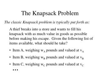
The Knapsack Problem • Instance: • Multiset of integers • Capacity • Find:
SimpleAlgorithms & Analysis • Incremental Insertion (II) • Arbitrary order • Increasing order • Decreasing order (Greedy) • Local Exchange (LE) • PTASing • “Optimal Head – Greedy Tail” (GRT)
II – Arbitrary Order • Go over the elements (arbitrary order) • Insert an element if the capacity not exceeded • Theorem:
Proof • Suppose the weights are • Let be any locally optimal solution • We may assume • Otherwise, is optimal
Proof(cont.) • Let be the largest index of a weight not belonging to Since is locally optimal
Proof(cont.) • Denote by the interval • For any solution not containing • Either • Or • That is, the number of solutions with total weight in is at most
Proof(cont.) • Solutions of weight at least are infeasible. • Solution weighted not more than are not better than
Proof(cont.) • Blackball instance: • II can lead to • Which is locally optimal blackball
Proof(cont.) • Taking the first item and omitting at least one of the rest is better. • Hence • And we finished...
II – Increasing Order • No Gain! • That was our blackball… • In the previous proof.
II - Decreasing Order (Greedy) • No drastic gain! • Blackball instance B: blackball
II - Decreasing Order (Greedy) • Greedy(B) • Weight: • Any solution taking • Exactly two elements from • Any of the last elements is better!
SimpleAlgorithms & Analysis • Incremental Insertion (II) • Arbitrary order • Increasing order • Decreasing order (Greedy) • Local Exchange (LE) • PTASing • “Optimal Head – Greedy Tail” (GRT)
Local Exchange (LE) • Assume is a solution • Allowed operations: • Insert a new element x to • Exchangex by y • x belongs to • y not belongs to • x < y
Local Exchange • Theorem:
Proof • Suppose the weights are • Let be any locally optimal solution • We may assume • Otherwise, is optimal
Proof(cont.) • Let be the largest index of a weight not belonging to Since is locally optimal
Proof(cont.) • Denote by the interval • For any solution not containing • Either • Or • That is, the number of solutions with total weight in is at most • And there are at least outside
Proof(cont.) • Let be the number of items belonging to among the first k -1 items • Let be the number of items not belonging to among the first k -1 items • How many solution pairs are of weight not belonging to ?
Proof(cont.) • We saw that • All solutions obtained by dispensing of some items from And the one obtained from them by adjoining the ’th item not belong to the interval
Proof(cont.) • So • For each of the solutions obtained from by adjoining one of the items of • Both the obtained solution • And the one obtain by adjoining it the ’th item not belong to the interval
Proof(cont.) • So • Since our solution can not be improved by local exchange • Each of the n-k solutions obtained by removing one of the last n-k items not belong to the interval • Adding each of them the ’th item we get infeasible solutions
Proof(cont.) • So
Proof(cont.) • Blackball instance: • LE can lead to • Which is locally optimal blackball
Proof(cont.) • Taking the first item and omitting at least two of the rest is better. • Hence: • And we finished... b(n)
SimpleAlgorithms & Analysis • Incremental Insertion (II) • Arbitrary order • Increasing order • Decreasing order (Greedy) • Local Exchange (LE) • PTASing • “Optimal Head – Greedy Tail” (GRT)
PTASing • There exist a PTAS for Knapsack • That is, it is possible to approximate the optimal solution to within any factor c >1 • In time polynomial in n and 1/(c -1) • We’ll see
Theorem 1 • Let be an instance of KP • Denote the weight of optimal solution by • Assume H is a factor-c approximation for KP • Then
Proof • Assume that the elements of optimal solution are labeled such that • Let ’ be the smallest integer such that