Download
1 / 44
440 likes | 477 Views
TerraFlow offers automatic estimation of terrain parameters, such as watersheds, drainage networks, and topographic indices. This collection of programs models flow direction and accumulation on large grids with optimal efficiency, scalability, and flexibility, making it 2-1000 times faster than existing software. Learn about local vs. scattered data access and the importance of disk I/O speed for analyzing massive grids.

E N D
Digital Terrain Analysis for Massive Grids Lars Arge, Jeff Chase, Laura Toma, Jeff Vitter, Rajiv Wickremesinghe Pat Halpin, Dean Urban in collaboration with http://www.cs.duke.edu/geo*/terraflow
Modeling Flow Sierra-Nevada DEM Flow Direction Flow Accumulation
Flow direction The direction water flows at a cell Flow Routing Compute flow direction for all cells in the grid Flat areas Flooding Flow accumulation value Total area which flows through a cell in the terrain per unit width of contour Flow Accumulation Compute flow accumulation values for all cells in the terrain Flow is distributed according to the flow directions Modeling Flow
Automatic estimation of terrain parameters watersheds drainage networks topographic index Surface saturation Soil water content Erosion, Deposition Forest structure Species diversity Sediment transport Applications
Massive Data • Remote sensing data available today • USGS (entire US at 10m resolution) • NASA-SRTM (whole Earth 5TB at 30m resolution) • Higher resolution data available • Ex: Appalachian Mountains dataset • 100m resolution (500MB) • 30m resolution (5.5GB) • 10m resolution (50GB) • 1m resolution (5TB)
Problems with Existing Software • GRASS • r.watershed • Killed after17 days on a 50MB dataset • TARDEM • flood, d8, aread8 • Can handle the 50MB dataset • Killed after running for 20 days on a 130MB dataset • CPU utilization: 5%, 3GB swap file • ArcInfo • flowdirection, flowaccumulation • Can handle the 130MB dataset • Doesn’t work for files bigger than 2GB
Our Results: TerraFlow • Collection of programs for flow routing and flow accumulation on massive grids • Theoretical results • Flow routing and flow accumulation modeled as graph problems and solved in optimal bounds • Practical results • Efficient • 2-1000 times faster than existing software on massive grids • Scalable • 1 billion elements!! (>2GB data) • Flexible • Outputs similar with ArcInfo flowdirection and flowaccumulation http://www.cs.duke.edu/geo*/terraflow
Scalability: Why? How? Massive data • Data does not fit in memory • OS places data on disk and moves data in and out of memory • Data is moved in blocks • Accessing disk is 1000 times slower than accessing main memory disk I/O is the bottleneck! Local data accesses vs. scattered data accesses l
1 2 5 6 9 10 3 4 7 8 Local Accesses vs. Scattered Accesses • Example: reading an array from disk • Array size N = 10 elements • Disk block size = 2 elements • Memory size = 4 elements (2 blocks)
1 2 5 6 9 10 3 4 7 8 Local Accesses vs. Scattered Accesses • Example: reading an array from disk • Array size N = 10 elements • Disk block size = 2 elements • Memory size = 4 elements (2 blocks)
1 2 5 6 9 10 3 4 7 8 Local Accesses vs. Scattered Accesses • Example: reading an array from disk • Array size N = 10 elements • Disk block size = 2 elements • Memory size = 4 elements (2 blocks)
1 2 5 6 9 10 3 4 7 8 Local Accesses vs. Scattered Accesses • Example: reading an array from disk • Array size N = 10 elements • Disk block size = 2 elements • Memory size = 4 elements (2 blocks)
1 2 5 6 9 10 3 4 7 8 Local Accesses vs. Scattered Accesses • Example: reading an array from disk • Array size N = 10 elements • Disk block size = 2 elements • Memory size = 4 elements (2 blocks)
1 2 5 6 9 10 3 4 7 8 Local Accesses vs. Scattered Accesses • Example: reading an array from disk • Array size N = 10 elements • Disk block size = 2 elements • Memory size = 4 elements (2 blocks)
1 2 5 6 9 10 3 4 7 8 Local Accesses vs. Scattered Accesses • Example: reading an array from disk • Array size N = 10 elements • Disk block size = 2 elements • Memory size = 4 elements (2 blocks)
1 2 5 6 9 10 3 4 7 8 Local Accesses vs. Scattered Accesses • Example: reading an array from disk • Array size N = 10 elements • Disk block size = 2 elements • Memory size = 4 elements (2 blocks)
1 2 5 6 9 10 3 4 7 8 Local Accesses vs. Scattered Accesses • Example: reading an array from disk • Array size N = 10 elements • Disk block size = 2 elements • Memory size = 4 elements (2 blocks)
1 2 5 6 9 10 3 4 7 8 Local Accesses vs. Scattered Accesses • Example: reading an array from disk • Array size N = 10 elements • Disk block size = 2 elements • Memory size = 4 elements (2 blocks)
1 2 5 6 9 10 3 4 7 8 Local Accesses vs. Scattered Accesses • Example: reading an array from disk • Array size N = 10 elements • Disk block size = 2 elements • Memory size = 4 elements (2 blocks)
1 2 5 6 9 10 3 4 7 8 Local Accesses vs. Scattered Accesses • Example: reading an array from disk • Array size N = 10 elements • Disk block size = 2 elements • Memory size = 4 elements (2 blocks) Loads 5 blocks
1 2 10 9 5 6 4 3 8 7 1 5 2 6 3 8 9 4 7 10 Local Accesses vs. Scattered Accesses • Example: reading an array from disk • Array size N = 10 elements • Disk block size = 2 elements • Memory size = 4 elements (2 blocks) Loads 5 blocks
1 2 10 9 5 6 4 3 8 7 1 5 2 6 3 8 9 4 7 10 Local Accesses vs. Scattered Accesses • Example: reading an array from disk • Array size N = 10 elements • Disk block size = 2 elements • Memory size = 4 elements (2 blocks) Loads 5 blocks
1 2 10 9 5 6 4 3 8 7 1 5 2 6 3 8 9 4 7 10 Local Accesses vs. Scattered Accesses • Example: reading an array from disk • Array size N = 10 elements • Disk block size = 2 elements • Memory size = 4 elements (2 blocks) Loads 5 blocks
1 2 10 9 5 6 4 3 8 7 1 5 2 6 3 8 9 4 7 10 Local Accesses vs. Scattered Accesses • Example: reading an array from disk • Array size N = 10 elements • Disk block size = 2 elements • Memory size = 4 elements (2 blocks) Loads 5 blocks
1 2 10 9 5 6 4 3 8 7 Local Accesses vs. Scattered Accesses • Example: reading an array from disk • Array size N = 10 elements • Disk block size = 2 elements • Memory size = 4 elements (2 blocks) 1 5 2 6 3 8 9 4 7 10 Loads 5 blocks
1 2 10 9 5 6 4 3 8 7 1 5 2 6 3 8 9 4 7 10 Local Accesses vs. Scattered Accesses • Example: reading an array from disk • Array size N = 10 elements • Disk block size = 2 elements • Memory size = 4 elements (2 blocks) Loads 5 blocks
1 2 10 9 5 6 4 3 8 7 1 5 2 6 3 8 9 4 7 10 Local Accesses vs. Scattered Accesses • Example: reading an array from disk • Array size N = 10 elements • Disk block size = 2 elements • Memory size = 4 elements (2 blocks) Loads 5 blocks
1 2 10 9 5 6 4 3 8 7 1 5 2 6 3 8 9 4 7 10 Local Accesses vs. Scattered Accesses • Example: reading an array from disk • Array size N = 10 elements • Disk block size = 2 elements • Memory size = 4 elements (2 blocks) Loads 5 blocks
1 2 10 9 5 6 4 3 8 7 1 5 2 6 3 8 9 4 7 10 Local Accesses vs. Scattered Accesses • Example: reading an array from disk • Array size N = 10 elements • Disk block size = 2 elements • Memory size = 4 elements (2 blocks) Loads 5 blocks
1 2 10 9 5 6 4 3 8 7 1 5 2 6 3 8 9 4 7 10 Local Accesses vs. Scattered Accesses • Example: reading an array from disk • Array size N = 10 elements • Disk block size = 2 elements • Memory size = 4 elements (2 blocks) Loads 5 blocks
1 2 10 9 5 6 4 3 8 7 1 5 2 6 3 8 9 4 7 10 Local Accesses vs. Scattered Accesses • Example: reading an array from disk • Array size N = 10 elements • Disk block size = 2 elements • Memory size = 4 elements (2 blocks) Loads 5 blocks
1 2 10 9 5 6 4 3 8 7 1 5 2 6 3 8 9 4 7 10 N N blocks blocks << B Local Accesses vs. Scattered Accesses • Example: reading an array from disk • Array size N = 10 elements • Disk block size = 2 elements • Memory size = 4 elements (2 blocks) Loads 5 blocks Loads 10 blocks
Scalability: Why? How? Massive data • Data does not fit in memory • OS places data on disk and moves data in and out of memory • Data is moved in blocks • Accessing disk is 1000 times slower than accessing main memory disk I/O is the bottleneck! Local data accesses vs. scattered data accesses • N/B << N block transfers However good the OS, it cannot change the data access pattern of the program!
TerraFlow Approach Improve locality by redesigning algorithms • Block size at least 8KB (32KB, 64KB) • Compute on whole block while it is in memory • Avoid loading a block each time • Speedup = block size! • I/O-Efficient algorithms http://www.cs.duke.edu/geo*/terraflow
Related Work • TerraFlow’s emphasis • Computational aspects, not modeling • Flow modeling • [O’Callaghan and Mark 1984] • D8 method for flow accumulation • [Jenson and Domingue 1988] • General technique of flooding • Existing software • ArcInfo, GRASS, Tardem, Topaz, Tapes-G, RiverTools
Flow Routing on Flat Areas …no obvious flow direction
TerraFlow Outline • Flow routing • Flood the terrain to eliminate sinks • Identify watersheds and construct watershed graph • Collapse watershed graph and raise sinks • Flow accumulation • Sweep terrain top-down to distribute flow • All these steps can be solved I/O-Efficiently http://www.cs.duke.edu/geo*/terraflow
Datasets http://www.cs.duke.edu/geo*/terraflow
TerraFlow v.s. ArcInfo http://www.cs.duke.edu/geo*/terraflow
Significant speedup over ArcInfo for large grids East-Coast dataset ArcInfo: 78 hours TerraFlow: 8.7 hours Washington State dataset TerraFlow: 63 hours ArcInfo: Cannot process files larger than 2GB! TerraFlow – Performance http://www.cs.duke.edu/geo*/terraflow
TerraFlow Features • Flow directions, Flow accumulation • SFD (single flow directions) • MFD (multiple flow directions) (SFD,SFD), (MFD,MFD), (MFD,MFD) • Flow accumulation • Use MFD and switch to SFD when flow value exceeds an user-defined threshold http://www.cs.duke.edu/geo*/terraflow
TerraFlow: Result samples http://www.cs.duke.edu/geo*/terraflow
TerraFlowResults Samples http://www.cs.duke.edu/geo*/terraflow
Conclusions / Future Work • TerraFlow - Flow modeling • More features • Modeling • New applications http://www.cs.duke.edu/geo*/terraflow http://www.cs.duke.edu/geo*/terraflow http://www.cs.duke.edu/geo*/terraflow