Download
1 / 21
210 likes | 351 Views
Coupling ROMS and CSIM in the Okhotsk Sea. Rebecca Zanzig University of Washington November 7, 2006. Outline. Motivation ROMS Configuration CSIM Model Specifications Coupling Between Models Heat and Freshwater Fluxes Surface stresses Preliminary Results Future Work. Motivation.

E N D
Coupling ROMS and CSIM in the Okhotsk Sea Rebecca Zanzig University of Washington November 7, 2006
Outline • Motivation • ROMS Configuration • CSIM Model Specifications • Coupling Between Models • Heat and Freshwater Fluxes • Surface stresses • Preliminary Results • Future Work
Motivation • To couple a terrain-following regional ocean model (ROMS) with a state-of-the-art ice model (CSIM). • Apply this new model configuration to the Sea of Okhotsk, which is the formation region for North Pacific Intermediate Water. • Investigate the deep water formation in the region and the impact of sea ice on it. • Investigate the impact of tides on sea ice.
Grid Setup • Resolution: • 43-63 N, 135-165 E • 16-23 km resolution • 20 vertical levels • ETOPO5 Bathymetry • 3000 meter maximum depth • East, South and West open boundaries* * Open boundary forcing thanks to the North Pacific model by Al Hermann and Liz Dobbins at PMEL
CPP Options • LMD interior mixing • KPP surface and bottom boundary layer mixing • Splines • Third-order upstream bias horizontal advection of tracers • Surface salinity flux correction • Open Boundaries (East, South and West) • Chapman free-surface condition • Flather 2D-momentum condition • Radiation condition for 3D-momentum and tracers
Forcing Data • Coordinated Ocean-ice Reference Experiments (CORE) dataset • 6 hourly • Winds • Relative Humidity • Sea level pressure • Sea level air temperature • Daily • Incoming shortwave radiation • Incoming longwave radiation • Monthly • Precipitation (Rain and Snow) • World Ocean Atlas
Community Climate System Sea Ice Model (CSIM) • Dynamic and Thermodynamic ice model • Elastic- Viscous- Plastic Dynamics • Supports Multiple ice types • Used in CCSM- global climate model • Modified to run in regional applications • Capable of computing fluxes over both ice and the open ocean
Raw input forcing data Modified forcing Surface Stresses Heat Fluxes ROMS & CSIM Coupling ROMS CSIM Freshwater Fluxes
Terrain–Following Issues: Frzmlt level at_hminat_hmax 20 0.000 0.000 19 -0.500 -2.855
Terrain–Following Issues: Frzmlt Temp < -1.8 ºC Temp > -1.8 ºC Temp > -1.8 ºC
Results - Percent Ice Coverage 3 year mean ~30 year mean
Scherbina et al (2004) • Data along northwestern shelf from 2 bottom moorings and a hydrographic survey in September 1999 • Factors thought to be important to dense water formation: • Location of the tidal mixing front • Baroclinic instability could stop dense water formation
Bottom Temperature
Density Section
Temperature Section
Future Work • Add tides to the simulation • Refine resolution • Interannual variability (not just climatological forcing) • Examine ventilation and deep water formation • Include the Amur River in simulation