Download
1 / 14
140 likes | 286 Views
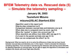
BFEM Telemetry data vs. Rescued data (5) -- Simulate the telemetry sampling --. Algorithm used in this report (p.2) Step-by-step comparison (p.3) Comparison between rescued data and telemetry one (p.4) When data size is compared event by event. (pp.5-6)

E N D
BFEM Telemetry data vs. Rescued data (5)-- Simulate the telemetry sampling -- • Algorithm usedin this report (p.2) • Step-by-step comparison (p.3) • Comparison between rescued data and telemetry one (p.4) • When data size is compared event by event. (pp.5-6) • When the “packet” is taken into account (pp.7-8) • When downlink rate differs from DAQ->BIU rate (pp.9-11) • # of event in the packet and data size (pp.12-13) • How can we compensate the effect? (p.14) January 06, 2003 Tsunefumi Mizuno mizuno@SLAC.Stanford.EDU Background: What we need to do is to solve the difference of data size we have found between rescued data and telemetry one. In this report, I tried to simulate the telemetry sampling algorithm. If we succeed in reproducing the telemetry data during ascent (Run54) by applying algorithm to rescued data, we are able to apply the algorithm to simulation and compare the results with level flight data (Run55).
Telemetry sampling algorithm • In this report, I simulate the telemetry sampling algorithm JJ and Tony taught me and see how it reproduces the data. The algorithm was applied to the rescued data and the results were compared with the telemetry data. The followings are the algorithm I have used in this report. • 1) DAQ takes events in bundles of 10 (i.e., “packet”)and applies the following algorithm. • 2) Event rate from DAQ to BIU (Balloon Interface Unit) is limited below 25kBytes/s (=R1). To do this, earned bytes (we call this “balance”) is calculated as below • balance (current) = balance (previous) + 25kBytes/s * deltaT • Here, deltaT is the arrival time difference of the last event in current packet and the previous one. Arrival times are in unit of 0.01s (= clock cycle of TEM) • If balance exceeds 25kBytes, it is reduced down to 25kBytes. This is to prevent the “burst” of DAQ after the long time interval. • 3) Next, calculate how many events (“num”) DAQ can send to BIU as below. • num = balance/(average event size of this packet) • 4) If the “num” is 1, compare the size of the 1st event in the packet with the balance. If the “num” is 2, compare the size of the 1st event and then that of 6th event with the balance. If the “num” is 3, 1st, 4th, 7th, ….. • 5) If the event size is smaller than the balance, send the event to BIU and subtract the size from the balance and go to the next event. Once the event size is larger than the balance, quit comparison and go to the next packet. • 6) BIU has its own limitation of event rate (=R2) and this might differ from R1. I first assumed that R2 is 25kBytes/s (accept all events from DAQ), and then tried another value (pp. 9-11).
Step-by-step comparison • In order to see how the algorithm affects the data property (especially event size distribution), they will be applied not at once but step by step as follows. • In page 4, no algorithm is applied and rescued data are compared with telemetry one directly. • Next, in pages 5-6, every except item 1 in page 2 is taken into account (i.e., data size is compared with balance for every event). • Then, all algorithm (items 1-5 in page2) is applied to rescued data and results are compared with telemetry one in pages 7-8. Note that R2 is assumed to be equal to R1. • After that, allow R2 different from R1 (pages 9-11). • The data used are rescued data of run #0 (the lowest trigger rate), #2 (trigger rate is close to that of level flight) and #5 (the highest trigger rate). See the figure below. Figure 1: L1T count rate of Run54 (during ascent). Run54 consists of 16 small runs, and run#0, #2, #3, #5 and #6 are recovered from the disk (i.e., rescued data). #5 #6 #3 #2 #0
Direct comparison between rescued data and telemetry data (run #0 in Run54) (run #2 in Run54) (run #5 in Run54) telemetry data rescued data Figure 2: TKR data size distribution of telemetry data and rescued one. Top panels show overall distribution and bottom ones show expanded distribution. I have already shown them in previous report and put them here again for reference.
Comparison between rescued data with sampling algorithm and telemetry one: data size is compared for every event (1) (TKR data size) (spacing of event#) (run #0 in Run54) telemetry data rescued data with algorithm Figure 3: TKR data size (left panels), spacing of event number (upper right) and deltaT (lower right) distribution of run #0 in Run54. The latter two figure show difference between rescued data with algorithm and telemetry data. (deltaT) (TKR data size)
Comparison between rescued data with sampling algorithm and telemetry one: data size is compared for every event (2) (TKR data size) (spacing of event#) (run #2 in Run54) telemetry data Figure 4: The same as Figure 3 but for run #2 instead of run #0. Right two figures show difference between rescued data with algorithm and telemetry data like Figure3. TKR data size also differs between them: when we compare event size and “balance” event by event, average data size becomes smaller than that of telemetry data. rescued data with algorithm (TKR data size) (deltaT) • As already reported, just comparing data size with “balance” for every event is not enough to reproduce telemetry data: it failed to reproduce the quantization in spacing of event number, it gave narrower deltaT distribution, and, most importantly, it gave smaller data size. In pages 7 and 8, we examine whether they are solved or not by taking “packet” (item 1 in page 2) into account.
Comparison between rescued data with sampling algorithm and telemetry one: “packet” is taken into account (1) (TKR data size) (run #0 in Run54) (spacing of event#) telemetry data Figure 5: TKR data size (left panels), spacing of event number (upper right) and deltaT (lower right) distribution of run #0 in Run54, where all (items 1-5 in page2) are taken into account. R2 is assumed to be the same as R1. Although small difference is seen in right two panels, situation is much improved (please compare with Figure3). rescued data with algorithm (TKR data size) (deltaT)
Comparison between rescued data with sampling algorithm and telemetry one: “packet” is taken into account (2) (spacing of event#) (TKR data size) (run #2 in Run54) telemetry data Figure 6: The same as Figure 5 but for run #2 in Run54 instead of run #0. rescued data with algorithm (deltaT) (TKR data size) • We got much improved distribution by taking “packet” into account (good news). Nevertheless, we still failed to reproduce the data size distribution when trigger rate is high. We also could not reproduce the double-peak in deltaT distribution. This makes us uneasy, because it might affect the event size distribution. Next step is to allow downlink rate different from DAQ->BIU rate (item 6 in page 2). Please go to pages 9-11.
Comparison between rescued data with algorithm and telemetry one: downlink rate is different from DAQ->BIU rate (1) • Downlink rate (R2 in page2) might differ from DAQ->BIU rate (R1). What is the value of R2? Average event size (includes not only TKR but also CAL, ACD, etc.) is about 1840 Byte and observed telemetry event rate is about 12Hz. Thus, R2 might be 1840*12/1024=21.6kHz. In pages 9-11, R2 is assumed to be 21.6kHz. (TKR data size) (spacing of event#) (run #0 in Run54) telemetry data Figure 7: TKR data size (left panels), spacing of event number (upper right) and deltaT (lower right) distribution of run #0 in Run54, where all (items 1-5 in page2) are taken into account and R2 is 21.6kHz instead of 25kHz (item 6 in page2). rescued data with algorithm (TKR data size) (deltaT) • It’s perfect! Now we are confident that we succeeded in simulating the telemetry sampling algorithm. Then, how well we can reproduce run #2 and run #5? Please go to pages 10 and 11.
Comparison between rescued data with algorithm and telemetry one: downlink rate is different from DAQ->BIU rate (2) (TKR data size) (spacing of event#) (run #2 in Run54) telemetry data Figure 8: The same as Figure 7 but for run #2 in Run54 instead of run #0. rescued data with algorithm (TKR data size) (deltaT)
Comparison between rescued data with algorithm and telemetry one: downlink rate is different from DAQ->BIU rate (3) (TKR data size) (spacing of event#) (run #5 in Run54) telemetry data Figure 9: The same as Figure 7 but for run #5 in Run54 instead of run #0. rescued data with algorithm (deltaT) (TKR data size) • Although deltaT distribution looks OK, we still see difference in the TKR data size distribution (lower left panel in Figure8 and 9). What causes this difference? The key could be in distribution of event# spacing. Although the number of events in packet was usually 10, it became 9 or less occasionally for some reason, as shown by black histogram in upper right panels of Figure 8 and 9. In next page, we will examine how this affects the data size distribution.
# of events in packet and TKR data size (1) (run #0 in Run54) The first event in the packet, where # of events in the previous packet is 9 previous event (i.e., the last event in the previous packet) all events in rescued data Figure 10: The TKR data size distribution of run #0 in Run54. The first event in the packet and the previous event are shown, where the number of events in the previous packet is 9. All events in rescued data are also given for reference. • Here, I picked up small packet (the number of events is 9) and plot the TKR data size distribution of the last event in this packet (blue histogram, not downlinked via telemetry) and the next one (green histogram, downlinked). As we can see, when the number of events in the packet is less than 10, the first event in the next packet shows small data size. Considering that most of downlinked events are the first event in the packet, this could be the reason why telemetry data shows smaller event size distribution as seen in left panels in Figure 8 and 9. smaller size previous packet (# of events=9) current packet
# of events in packet and TKR data size (2) (run #2 in Run54) The first event in the packet, where # of events in the previous packet is 10 previous event (i.e., the last event in the previous packet) all events in rescued data Figure 11: The TKR data size distribution of run #2 in Run54. The first event in the packet and the previous event are shown, where the number of events in the previous packet is 10. All events in rescued data are also given for reference. • How does the run#2 (trigger rate is ~500Hz) look like? In this case, we do not know the number of event of each packet (right?). Instead, I here selected events where the spacing of event number is multiples of 10. Then, the number of events in the previous packet should be 10. We thus obtained the figures above. The green histogram is consistent with the red one. Thus, if the # of events in the previous packet is 10, the size of the first event in the current packet is no longer smaller than others. On the other hand, the last event in the previous packet (blue histogram) shows larger data size distribution. Therefore, I suspect that, (a) if the size of 10th event is relatively large, this event is likely to be included in the current packet (# of events in the packet is 10), and (b) if it is relatively small, this event is likely to be included in the next packet (# of events in the packet becomes 9) and this causes smaller event size distribution seen in Figure 8 and 9. larger size normal size previous packet (# of events=10) current packet
How can we compensate the influence on data size? • We saw that # of events in the packet affects the data size. Since we have already succeeded in simulating the telemetry sampling, all we have to do is to compensate this effect. How can we do this? Generally speaking, there are two ways. • To pick up events where the # of events in the previous packet is 10. Unfortunately, we do not know the # of events in each packet (right?). Instead, we can select events where the spacing of event # is multiples of 10. One drawback of this method is that number of events we can use is reduced from 100k down to ~30k, as shown in Figure 12. • To figure out the mechanism to make # of events in packet less than 10 and simulate it. Though, I am afraid that this is not as easy as what we have done so far. Figure 12: Distribution of spacing of event# of Run55 (level flight). If we require that the spacing is multiples of 10, the number of events is reduced from ~100k to ~30k.