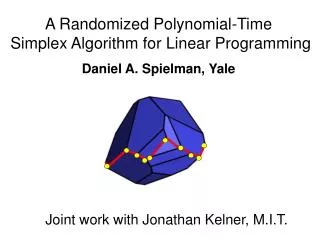
A Randomized Polynomial-Time Simplex Algorithm for Linear Programming

A Randomized Polynomial-Time Simplex Algorithm for Linear Programming Daniel A. Spielman, Yale Joint work with Jonathan Kelner, M.I.T.

Linear Programming maximize where is a n x d matrix, Rn Terminology: c = objective function b= right-hand side vector A has rows a1,…,an subject to

Linear Programming Algorithms • 1940s—Dantzig, simplex method • First practical method for solving linear programs • Runs efficiently in practice on most problems • No known variant ran in worst-case poly time • 1979—Khachiyan, Ellipsoid • Poly time, but usually slower than simplex • 1984—Karmarkar, Interior Point Methods • Poly time, sometimes slower than simplex, • sometimes faster

Simplex Methods Typically, walk on vertices and edges of feasible polytope Not known if graph on vertices and edges has polynomial diameter (See Kalai-Kleitman) Simplex methods have been generalized to walk on more general graphs. Ex.: Self-dual simplex (Dantizg, Lemke), Criss-cross, Admissible pivots (See Fukuda-Lüthi-Namiki)

Main Result A Randomized Polynomial-Time LP Simplex Method polynomial dependence on bit-length No bound on diameters of polytopes Walks on perturbations of polytopes generated from original LP problem A worst-case analysis inspired by Smoothed Analysis (S-Teng),

Overview 1. Reduce to problem of certifying boundedness 2. Boundedness does not depend on RHS, 3. Perturb , and run shadow-vertex simplex on perturbed polytope to generate certificate of boundedness 4. If fail, adjust distribution on perturbations, and try again.

Certifying Boundedness Unbounded if feasible region contains a ray in direction such that Unbounded iff all s lie in a halfspace Certify boundedness by expressing origin as a full-dimensional convex combination of the s

Reduction to certifying boundedness Recall dual LP: Combine primal and dual so that just need feasible Standard reduction to certifying boundedness, removing degeneracy by deterministic perturbation (See Megiddo-Chandrasekaran)

Boundedness Certification Problem Need to show origin in To apply simplex method, consider polytope Boundedness independent of , so can perturb Find certificate by optimizing random and , using shadow-vertex simplex method

Perturbing Walking on perturbed polytope is the same as walking on possibly infeasible vertices of original polytope

The Shadow Vertex Pivot Rule Simplex methods easy in 2d Feasible region is a polygon Possible pivot rules are “clockwise” and “counterclockwise” Lift this simplicity to higher-dimensional LPs

The Shadow of a Polytope Vertices  Vertices, Edges  Edges

The Shadow Vertex Pivot Rule start objective Vertices in shadow = those optimizing objective functions in shadow plane

Well-Rounded Polytopes Definition: A polytope is k-well-rounded if where = radius r ball centered at origin

Perturbing a Well-Rounded Polytope Given k-well-rounded polytope Perturb, to get Where riare exponential rand vars with expectation 1/n:

Perturbing a Well-Rounded Polytope Theorem: For a uniform random shadow plane V, Expected number edges of shadow of onto V is at most Where, P is k-well-rounded,

Proof of well-rounded shadow bound Expected length of perimeter of shadow of is < For every potential edge, given that it appears on the shadow, expected length of its shadow is > So, expect at most edges

Expected length of edge on shadow An edge is determined by the set of d-1 constraints that are tight on it For each , let be event that it appears on the convex hull of Q and in the shadow on V. If appears in shadow, let  be its length Lemma:

Expected length of edge on tope For each , let be event that it appears on the convex hull of Q. If appears, let be its length Lemma:

Arbitrarily set ri for all Consider line L of points satisfying aiTx=1+ri for all Every other constraint intersects this line either positively or negatively Edge length is distance between intersection points of max neg. constraint and min pos. constraint Proof: Expected length edge on tope

Proof: Expected length edge on tope As perturb , intersection point moves by at least size of perturbation Small edge unlikely now follows from memoryless property of exponential distribution:

Proof: Expected length of shadow edge Projection unlikely to decrease edge length too much Let be angle of edge to V. Lemma: Remark: Simple if do not condition upon

Proof: Expected length of shadow edge Lemma: To condition on , Note in shadow iff V intersects So, parameterize V by point in and a point orthogonal to that Compute integral in these new variables

Obstacles to obtaining algorithm Cannot use random 2-plane: Must have start vertex and objective function. Resolve by planting start vertex, and slightly extending theorem. Polytope is not necessarily well-rounded. But, when fail, learn how to make it rounder.

Starting Insert a vertex optimizing a 1/poly ball around by adding d artificial constraints near Will become the start vertex Choose c from a 1/poly ball around Vertex optimizing c will not involve artificial constraints Observe that did not need uniform random 2-plane: only need polynomial randomness, so take span(c, v), where v is random.

If Not Well-Rounded Run algorithm as if it were well-rounded If do not go all the way around shadow, learn a point in polytope of large norm. Using this point, change probability distributions on r1, …, rn and V. Is like re-scaling. Only need to do number times polynomial in bit-length. Is only barrier to strongly-polynomial time.

If Not Well-Rounded Using this point, change probability distributions on r1, …, rn and V. Is like re-scaling.

Open Questions Strongly Polynomial Algorithm? Other Algorithmic Applications?

A Randomized Polynomial-Time Simplex Algorithm for Linear Programming