Microstructure-Properties: II Driving Forces for Phase Transformations

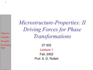
1. Microstructure-Properties: IIDriving Forces for Phase Transformations 27-302 Lecture 1 Fall, 2002 Prof. A. D. Rollett

2. Materials Tetrahedron Processing Performance Microstructure Properties

3. Objective • The objective of this lecture is to provide a quantitative description of the driving force(s) for phase transformations. • The overall direction is to describe phase transformations quantitatively and explain the basis of TTT and CCT diagrams for engineering use.

4. References • Phase transformations in metals and alloys, D.A. Porter, & K.E. Easterling, Chapman & Hall. • Stability of Microstructure in Metallic Systems, J.W. Martin, R.D. Doherty and B. Cantor, Cambridge Univ. Press. • Materials Principles & Practice, Butterworth Heinemann, Edited by C. Newey & G. Weaver. • Grain Boundary Migration in Metals, G. Gottstein and L.S. Shvindlerman, CRC Press (1999).

5. Nucleation & Growth • All phase transformations can be described as nucleation & growth processes. • In order to understand, predict and engineer phase transformations, we must understand the driving force, the kinetics and the mechanisms of transformations. • We have encountered one example of transformation, recrystallization, in 301. • In 302, we will concentrate on solid state transformations.

6. Driving Force • We assume familiarity with thermodynamic driving force. • Example: solidification: as you cool a liquid below the liquidus, so the driving force for solidification increases. This driving force is often called undercooling. • Example: precipitation: as you cool a single phase material below a solvus, so the driving force for precipitation increases. • Example: phase change: for a pure substance with more than one allotrope, as you cool it below the phase transformation temperature, so the driving force for the phase change increases.

7. Driving Force Equation Approx. Value Force (MPa) Stored energy of deformation 1/2rmb2 r~1015 10 Grain boundaries 2sb/R sb~0.5 J/m2 10-2 Surface energy 2Dss/d D~10-3m 10-4 Chemical driving force R(T1-T0)c0lnc0 5%Ag in Cu @ 300°C 10+2 Magnetic field m0H2Dc/2 H~107A/m 10-4 Elastic energy t2(1/E1-1/E2)/2 t~10 MPa 10-4 Temperature gradient DS 2lgradT/Wa l~5x10-10 10-5 Driving Forces - Examples

8. Real World Examples • Practical examples occur all over materials science & engineering. • If you cool below a single-phase Al-Ag (example from the exam) below the solvus for the Al2Ag phase then there is a driving force for the new phase to appear. • The existence of a thermodynamic driving force does not mean that the reaction will necessarily occur! For example, there is a driving force for diamond to convert to graphite but there is (huge) nucleation barrier (fortunately!). • A supercooled melt has a driving force for solidification to occur. Again, nucleation is required before it actually takes place. • Air (over-)saturated in water has a driving force for rain to occur. Depending on circumstances, the precipitation of water droplets may occur as a mist, i.e. fine enough droplets that they remain as a suspension in the air.

9. Quantitative Approach • Following P&E, pp 10-11, we can quantify the driving force for solidification (and allotropic phase change). • Assume that the free energies of the solid and liquid are approximately linear with temperature. MolarFreeEnergy ∆G GS GL ∆T Temperature TMelt

10. Driving force: solidification • Writing the free energies of the solid and liquid as:GS = HS - TSS GL = HL - TSL ∆G = ∆H - T∆S • At equilibrium, i.e. Tmelt, then the ∆G=0, so we can estimate the melting entropy as:∆S = ∆H/Tmelt = L/Tmeltwhere L is the latent heat (enthalpy) of melting. • Ignore the difference in specific heat between solid and liquid, and we estimate the free energy difference as: ∆G  L-T(L/Tmelt) = L∆T/Tmelt

11. Driving force: precipitation • The other case of interest is precipitation. • This is more complicated because we must consider the thermodynamics of solids with variable composition. • Consider the chemical potential of component B in phase alpha compared to B in beta. This difference, labeled as ∆Gn on the right of the lower diagram is the driving force (expressed as energy per mole, in this case). • To convert to energy/volume, divide by the molar volume for beta: ∆GV = ∆Gn/Vm. Te T P N R S Q U

12. Driving force for nucleation • It is important to realize the difference between the driving force for the reaction as a whole, which is given by the change in free energy between the supersaturated solid solution and the two-phase mixture, shown as ∆G0 in 5.3b (the distance N-S). • Why a different free energy for nucleation? Because the first nuclei of beta to appear do not significantly change the composition of the parent material. Thus the free energy change for nucleation is the rate of change of free energy for the new, product phase (beta).

13. Driving force, contd. • Based on the expression for the chemical potential of a component (P&E 1.68):µB = GB + RT lngBXB • We can identify the chemical potential for B in the supersaturated phase as µB0, and the chemical potential for B in precipitated beta in equilibrium with the alpha phase as µBe. Then the molar free energy difference, ∆Gn, (distance P-Q) is given by∆Gn = µB0 - µBe = RT ln(gB0XB0/gBeXBe). • We can simplify this for ideal solutions (g=1) or for dilute solutions (g=constant) to:∆Gn = RT ln(X0/Xe).

14. Details • A more detailed approach considers the ratios of the compositions of the phases in addition to the differences in chemical potential [Martin et al., p10-11]. • Consider fig. 5.3b again. The triangle R-P-Q is similar (mathematically) to the triangle R-T-U. • The decrease in free energy per mole of precipitate is the distance P-Q, which is smaller than the difference in chemical potential for B in the supersaturated material at X0 and in the beta precipitate at Xbeta.∆Gn = (µB0 - µBe){Xbeta-Xe}/{1-Xe} = RT ln(gB0XB0/gBeXBe) {Xbeta-Xe}/{1-Xe} .∆Gn = RT ln(X0/Xe) {Xbeta-Xe}/{1-Xe}. • However, for precipitate that is pure B (or close to that) the fraction in curly brackets,{Xbeta-Xe}/{1-Xe}, is close to one, hence the result given on the previous slide.

15. Examples • The driving force is very sensitive to the mole fractions of the precipitate, Xbeta,, supersaturated matrix, X0, and equilibrium matrix, Xe. • For a ratio Xe/X0 = 10-3, Xbeta=1, and a temperature of 300K (i.e. very low solubility at a low enough temperature), then the driving force is estimated to be -17,000 J/mole. For the precipitation of pure Cu from Al, for example, this is a feasible estimate. • For many precipitation reactions, the volume fraction of the precipitate, Vbeta= {X0 -Xe}/{Xbeta-Xe}, is of order 0.1, which means that the driving force is much less, ~ -1,700 J/mole. If the precipitate is not pure B, but incorporates a significant amount of A, as for example in Al6Mn, then there is a further reduction in the driving force.

16. Solid Solubility • Before we can proceed, however, we need to look at the variation in solubility with temperature. This variation can be quite complex, so we will simplify the situation (considerably) by considering a regular solid solution. See section 1.5.7 in P&E. In short, the solubility can often be approximated by an Arrhenius expression, where Q is the heat absorbed (enthalpy) when I mole of beta dissolves in A as a dilute solution.

17. Driving force as a function of temperature • Despite the complications of the previous analysis, the net result is startlingly simple. • The driving force is, to first order, proportional to the undercooling!

18. Nucleation Rate • Armed with this information about driving force (note that the proportionality to undercooling is the same as for solidification), we can now look at how the nucleation rate varies with temperature. • The energy barrier for nucleation varies as the square of the driving force: the nucleation rate is exponentially dependent on the barrier height.

19. Elastic energy effect • Elastic effects have the effect of offsetting the undercooling by ∆GS. • Diffusion limits the rate at which atoms can form a new phase and hence limits the nucleation rate at low temperatures.

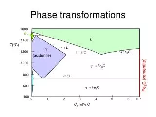
20. Allotropic Phase Transformations • These are, for example, eutectoid transformations (or peritectoid). • The calculation of driving force is similar: • Notation (e.g. Fe-C system):X0:= alloy composition (e.g. C in Fe) Xg:= equilibrium austenite composition Xa:= equilibrium ferrite composition • Driving force:∆Gn = {Xg- Xa}/XgRT ln{(1-Xg)/(1-X0)}. • For a typical case of T=1000K, Xg = 0.04, Xa = 0.001, X0:= 0.02 (equivalent to 0.4 weight % C), ∆Gn = -170 J/mole. This is much smaller than the previous estimates for precipitation. Homogeneous nucleation is essentially impossible!

21. Analogies for Driving Force • There are two obvious analogies for the driving force in phase transformation (in addition to the analogies to driving forces in grain growth and recrystallization). They are (1) water flow and (2) electricity. • Water flows from downhill (as we all know!). Height represents a measure of driving force. To be more accurate, the product of density, r, height and the acceleration due to gravity is equal to the pressure at the base of a column of fluid. p = h r g

22. Analogies: electric circuits • The other analogy is that of electric circuits (direct current). In this case, the voltage plays the role of pressure, also by analogy to water pressure. • According to Ohm’s Law, the current is equal to the voltage [pressure] divided by the resistance,I = V / R To continue the analogy with driving force and nucleation in phase transformation, however, would require a more complex circuit. There would have to be a component that responded non-linearly to applied voltage. In fact, varistors behave in this fashion: they pass very little current until a threshold voltage is exceeded and then they let large currents through. This effectively limits the maximum voltage that can be sustained across them.

23. Summary • For solidification, the driving force is proportional to the undercooling. • For the case of precipitation where the solid solubility is described by an ideal or regular solution, the driving force is also proportional to the undercooling. • The driving force is the information that we need in order to predict the nucleation rate.