Download
1 / 64
640 likes | 759 Views
Genome Rearrangements. CIS 667 April 13, 2004. Genome Rearrangements. We have seen how differences in genes at the sequence level can be used to infer evolutionary relations among species

E N D
Genome Rearrangements CIS 667 April 13, 2004
Genome Rearrangements • We have seen how differences in genes at the sequence level can be used to infer evolutionary relations among species • Differences in sequences in (one or more) genes resulted from point mutations (insert, delete, substitute) • These are not the only type of changes that can occur in the genome
Genome Rearrangements • Repair of broken chromosomes is an important process • Mistakes can occur, however • Mistakes can also occur during crossover • These mistakes cause changes in gene order • A large piece of chromosome can be moved or copied to another location • It can also move from one chromosome to another • We call these movements genome rearrangments
Genome Rearrangements • These have important (usually fatal) consequences for the organism and its evolution • Alignments do not capture genome rearrangments • Two species may have nearly the same gene sequences, but in a different order (why would the two species then be different?)
Genome Rearrangements • We need some other way to compare entire genomes (i.e. compare at a higher level) • Rather than simple point mutations a genome is obtained from another by a number of a special kind of rearrangements: Reversals • Use the number of reversals needed to transform one genome into another to measure evolutionary distance
The Method • Use combinatorial optimization techniques in an attempt to infer a most economical sequence of rearrangement operations to account for differences among the genomes • Compare with character-based methods for phylogenetics (parsimony)
Reversals • Consider the genome of a species as a sequence of blocks • A block is some sequence of the genome (possibly containing more than one gene) transcribed as a unit • Blocks are oriented since they can be transcribed from either strand of DNA • Give homologous blocks the same label
Reversals • Relation between chloroplast genomes of alfalfa and garden pea:
Reversals • Reversal operation for oriented blocks: • Inverts the order of affected blocks and changes their orientation (arrow) • Affects a contiguous segment of blocks • What sequence of reversal operations could have changed alfalfa into garden pea? • Would like to have a polynomial time algorithm to find the shortest sequence
Genome Comparison vs. Gene Comparison • In the late 1980s, J. Palmer and his colleagues studied the mitochondrial genomes of cabbage and turnips • The gene sequences are very similar (some genes are 99% equal) • Gene order, however, differs dramatically • Genome rearrangements are now considered to be a common mode of molecular evolution
Genome Comparison vs. Gene Comparison • Extreme conservation of genes on X chromosomes across mammalian species provides an opportunity to study the evolutionary history of X chromosome independently of the rest of the genomes • According to Ohno´s law, the gene content of X chromosome has barely changed throughout mammalian development in the last 125 million years. • However, the order of genes on X chromosomes has been disrupted several times.
Human and Mouse X Chromosomes -4 -6 1 7 2 -3 5 8 3 2 7 -1 6 4 5 8 1 7 2 -3 6 4 5 8 1 2 7 -3 6 4 5 8 1 2 7 3 -6 4 5 8 1 2 -5 -4 -3 6 7 8 1 2 3 4 5 6 7 8
Genome Comparison vs. Gene Comparison • The traditional molecular evolutionary technique is a gene comparison to construct a phylogenetic tree • In the ”cabbage and turnip” case this is hardly suitable, since rate of point mutations in their mitochondrial genes is so low that their genes are almost identical • Genome comparison (i.e. comparison of gene orders) is the method of choice in the case of very slowly evolving genomes • Another area is the case where genomes evolve very rapidly (genes not very similar)
Genome Comparison • Only about (17839) genome rearrangements have happened since human and mouse diverged 80 million years ago • Mouse and human genomes can be viewed as a collection of about 200 fragments which are shuffled in mice as compared to humans • A comparative mouse-human genetic map gives the position of a human gene given the location of a related mouse gene
Definitions • A signed permutation a over the set of labels L = {1, 2, …, n} is a permutation such that a(i) = +aor –a, where a Î L • Example: +3, –2, –1 is a signed permutation over L = {1, 2, 3} • Note that no label may appear twice in the permutation • A reversal [i,j] is an operation that transforms one signed permutation into another, reversing the order or a contiguous portion and flipping the signs
Definitions • a’ = a[i,j] = a(1), …, a(i – 1), –a(j), …, –a(i),a(j + 1), …, a(n) • We are interested in the problem of sorting by reversals: Given two signed permutations a and b, find the minimumnumber of reversals r1, …, rtthat will transform a into b - a r1…rt = b • The reversal distance db(a) = t
Definitions • Note that the reversal operation does not directly correspond to the biological operations (inversion, translocation, fission, fusion) • Given a and b, can we always transform a into b using only the reversal operation? If so, how many reversals are required in the worst case?
Breakpoints • A breakpoint is a point between consecutive labels in the initial permutation that must necessarily be separated by at least one reversal to reach the target permutation • The two consecutive labels are not consecutive in the target, or their orientations are not the same in a relative sense
Breakpoints • To formalize the idea of breakpoint, we introduce the extended version of a • Let a = a(1), …, a(n) • Then the extended version of a is (L, a(1), …, a(n), R) • For example let extended abe (L, –2, –3, +1, +6, –5, –4, R) and let extended b be (L, +1, +2, +3, +4, +5, +6, R) • The breakpoints are: (L,–2), (–2,–3), (–3,+1), (+1,+6), (6,–5), (–4,R)
Breakpoints • The number of breakpoints of a permutation a is denoted by b(a) • In the example, = 6 • Can you characterize the situations where L is involved in a breakpoint? When R is involved in a breakpoint?
A Lower Bound • A reversal can remove at most two breakpoints • Cuts the permutation in exactly two places • So, if ar1… rt = b then • b(a) – b(ar1) £ 2 • b(ar1) – b(ar1r2) £ 2 • … • b(ar1…rt-1) – b(ar1…rt) £ 2 • So b(a) £ 2t. If t = d(a), b(a)/2 £d(a)
Reality and Desire Diagram • The lower bound found is not very tight • We can derive a better l.b. based on a structure called the reality-desire diagram of a permutation with respect to another • To draw the diagram, we will represent +a with the tuple (-a +a) and -a with the tuple (+a -a) • The orientation is given by the rightmost member of the tuple
Reality and Desire Diagram • A permutation is a sequence of adjacent tuples: a = +3, –2, –1, +4, –5 can be represented as: L---(–3 +3)---(+2 –2)---(+1 –1)---(–4 +4)---(+5 –5)---R b = L---(–1 +1)---(–2 +2)---(–3 +3)---(–4 +4)---(–5 +5)---R
L -3 +3 +2 -2 +1 -1 -4 +4 +5 -5 R Reality and Desire Diagram • Now we will draw a graph to represent a (L, +3, -2, -1, +4, -5, R) • The reality diagram:
Reality and Desire Diagram • Suppose that b is the identity (L, +1, +2, +3, +4, +5) • We will add desire edges to the previous graph to represent b L -3 +3 +2 -2 +1 -1 -4 +4 +5 -5 R
Reality and Desire Diagram • a is the reality • b is what is desired • The diagram (a multigraph) shows both reality and desire • Call it RD(a) • We can rearrange the nodes of the graph to make it easier to understand
Reality and Desire Diagram L R Desire Reality
Properties of RD(a) • Each vertex has degree 2 • Each node is incident to one edge from A, the set of reality edges, and B, the set of desire edges • The connected components of the graph are alternating cycles (edges alternate between reality - blue - and desire - red) • Each cycle has an even number of edges, half reality and half desire
Properties of RD(a) • The number of cycles of RD(a) is denoted by cb(a) • Note that cb(b) = n + 1 since b has no breakpoints • All cycles are two parallel edges between the same pair of nodes • We have 2n + 2 nodes, so n + 1 cycles • This is the only permutation for which cb(a) = 1
Properties of RD(a) • So transforming a into b can be seen as transforming RD(a) into a graph with as many cycles as possible - n + 1 • Now we need to see how a reversal affects the cycles of RD(a) • Note that a reversal is characterized by the two points where it cuts the current permutation, which each correspond to a reality edge
Reversals and RD(a) • Let r be a reversal defined by two reality edges (s,t) and (u,v), then RD(ar) differs from RD(a) as follows: • Reality edges (s,t) and (u,v) are replaced by (s,u) and (t,v) • Vertices u, …, t are reversed • Desire edges remain unchanged • See example on following slide
Example Some nodes/edges omitted L L R R
Orientation of Cycles • How many cycles are affected by a reversal? • First we define convergent and divergent edges • Two reality edges on the same cycle converge if they are traversed in the same direction (clockwise or counterclockwise on the circle in the diagram) on the cycle • Otherwise they diverge
Orientation of Cycles L Convergent: (+3,+2) (-1,-4) Divergent: (L,-3) (+3,+2) R
Reversals and #Cycles • Let r be a reversal acting on two reality edges e and f • If e and f belong to different cycles, c(ar) = c(a) – 1 • If e and f belong to the same cycle and converge, c(ar) = c(a) • If e and f belong to the same cycle and diverge, c(ar) = c(a) + 1
First Case • If e and f belong to different cycles, c(ar) = c(a) – 1
Second Case • If e and f belong to the same cycle and converge, c(ar) = c(a)
Third Case • If e and f belong to the same cycle and diverge, c(ar) = c(a) + 1
Reversals and #Cycles • Note that the number of cycles changes by at most one with each reversal • Use that to find another lower bound for reversal distance • Suppose we have ar1r2…rt = b we know that c(b) = n + 1 and we have: • c(ar1) - c(a) 1 • c(ar1r2) - c(ar1) 1 • … • c(ar1r2…rt) - c(ar1r2…rt-1) 1 • Adding and cancelling terms we get • n + 1 - c(a) t • If r1r2…rtis optimal then t = d(a), n + 1 - c(a) d(a)
Interleaving Graph • This new lower bound is better than the old one - b(a)/2 • For most signed permutations, it is close to the actual distance, however it does not always work (we can’t always choose two divergent edges) • We can classify the cycles of RD(a) as good or bad: • A cycle is good if it has two divergent reality edges • Otherwise it is bad
Interleaving Graph • The classification only applies to proper cycles (those with at least four edges) • Those with three edges don’t need to be touched since reality = desire • If we have only good cycles in a permutation, then the lower bound previously given is an equality • We sort, increasing the number of cycles by one per reversal
Interleaving Graph • If a desire edge from one cycle crosses some desire edge from another cycle we say that the two cycles interleave • Interleaved cycles allow us to change a bad cycle into a good one while breaking another cycle • This good cycle can then broken in the next step • To find interleaving cycles, we construct an interleaving graph
Interleaving Graph • Nodes in the interleaving graph are cycles • Edge between two nodes if the cycles interleave • The connected components of the graph are called bad components if they consist entirely of bad cycles • Component otherwise is a good component
Interleaving Graph • What is the interleaving graph of the previous example? • Suppose that F and C are good cycles. • Which components of the interleaving graph are good and which are bad?