Download
1 / 123
1.35k likes | 1.94k Views
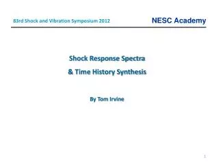
83rd Shock and Vibration Symposium 2012. Shock Response Spectra & Time History Synthesis By Tom Irvine. This presentation is sponsored by. NASA Engineering & Safety Center (NESC ). Dynamic Concepts, Inc. Huntsville, Alabama. Contact Information. Tom Irvine

E N D
83rd Shock and Vibration Symposium 2012 Shock Response Spectra & Time History Synthesis By Tom Irvine
This presentation is sponsored by NASA Engineering & Safety Center (NESC) Dynamic Concepts, Inc.Huntsville, Alabama
Contact Information Tom Irvine Email: tirvine@dynamic-concepts.com Phone: (256) 922-9888 The software programs for this tutorial session are available at: http://www.vibrationdata.com Username: lunar Password: module
Outline Response to Classical Pulse Excitation Response to Seismic Excitation Pyrotechnic Shock Response Wavelet Synthesis Damped Sine Synthesis MDOF Modal Transient Analysis
Classical Pulse Introduction • Vehicles, packages, avionics components and other systems may be subjected to base input shock pulses in the field • The components must be designed and tested accordingly • This units covers classical pulses which include: • Half-sine • Sawtooth • Rectangular • etc
Shock Test Machine • Classical pulse shock testing has traditionally been performed on a drop tower • The component is mounted on a platform which is raised to a certain height • The platform is then released and travels downward to the base • The base has pneumatic pistons to control the impact of the platform against the base • In addition, the platform and base both have cushions for the model shown • The pulse type, amplitude, and duration are determined by the initial height, cushions, and the pressure in the pistons platform base
Half-sine Base Input 1 G, 1 sec HALF-SINE PULSE Accel (G) Time (sec)
Systems at Rest Soft Hard Natural Frequencies (Hz): 0.063 0.125 0.25 0.50 1.0 2.0 4.0 Each system has an amplification factor of Q=10
Systems at Rest Soft Hard Natural Frequencies (Hz): 0.063 0.125 0.25 0.50 1.0 2.0 4.0
Responses at Peak Base Input Hard Soft Soft system has high spring relative deflection, but its mass remains nearly stationary Hard system has low spring relative deflection, and its mass tracks the input with near unity gain
Responses Near End of Base Input Soft Hard Middle system has high deflection for both mass and spring
Soft Mounted Systems • Soft System Examples: • Automobiles isolated via shock absorbers • Avionics components mounted via isolators • It is usually a good idea to mount systems via soft springs. • But the springs must be able to withstand the relative displacement without bottoming-out.
Isolated avionics component, SCUD-B missile. Public display in Huntsville, Alabama, May 15, 2010 Isolator Bushing
But some systems must be hardmounted. • Consider a C-band transponder or telemetry transmitter that generates heat. It may be hardmounted to a metallic bulkhead which acts as a heat sink. • Other components must be hardmounted in order to maintain optical or mechanical alignment. • Some components like hard drives have servo-control systems. Hardmounting may be necessary for proper operation.
Free Body Diagram Summation of forces
Derivation Equation of motion Let z = x - y. The variable z is thus the relative displacement. Substituting the relative displacement yields Dividing through by mass yields 19
Derivation (cont.) By convention is the natural frequency (rad/sec) is the damping ratio
Base Excitation Half-sine Pulse Equation of Motion Solve using Laplace transforms.
SDOF Example • A spring-mass system is subjected to: • 10 G, 0.010 sec, half-sine base input • The natural frequency is an independent variable • The amplification factor is Q=10 • Will the peak response be • > 10 G, = 10 G, or < 10 G ? • Will the peak response occur during the input pulse or afterward? • Calculate the time history response for natural frequencies = 10, 80, 500 Hz
SDOF Response to Half-Sine Base Input >> halfsine halfsine.m version 1.4 December 20, 2008 By Tom Irvine Email: tomirvine@aol.com This program calculates the response of a single-degree-of-freedom system subjected to a half-sine base input shock. Select analysis 1=time history response 2=SRS 1 Enter the amplitude (G) 10 Enter the duration (seconds) 0.010 Enter the natural frequency (Hz) 10 Enter amplification factor Q 10 maximum acceleration = 3.69 G minimum acceleration = -3.154 G Plot the acceleration response time history ? 1=yes 2= no 1
maximum acceleration = 3.69 G minimum acceleration = -3.15 G
maximum acceleration = 16.51 G minimum acceleration = -13.18 G
maximum acceleration = 10.43 G minimum acceleration = -1.129 G
Summary of Three Cases • A spring-mass system is subjected to: • 10 G, 0.010 sec, half-sine base input Shock Response Spectrum Q=10 Note that the Peak Negative is in terms of absolute value.
Half-Sine Pulse SRS >> halfsine halfsine.m version 1.5 March 2, 2011 By Tom Irvine Email: tomirvine@aol.com This program calculates the response of a single-degree-of-freedom system subjected to a half-sine base input shock. Assume zero initial displacement and zero initial velocity. Select analysis 1=time history response 2=SRS 2 Enter the amplitude (G) 10 Enter the duration (seconds) 0.010 Enter the starting frequency (Hz) 10 Enter amplification factor Q 10 Plot SRS ? 1=yes 2= no 1
SRS Q=10 10 G, 0.01 sec Half-sine Base Input X: 80 Hz Y: 16.51 G Natural Frequency (Hz)
Program Summary Papers sbase.pdf terminal_sawtooth.pdf unit_step.pdf Matlab Scripts halfsine.m terminal_sawtooth.m Video HS_SRS.avi
El Centro, Imperial Valley, Earthquake Nine people were killed by the May 1940 Imperial Valley earthquake. At Imperial, 80 percent of the buildings were damaged to some degree. In the business district of Brawley, all structures were damaged, and about 50 percent had to be condemned. The shock caused 40 miles of surface faulting on the Imperial Fault, part of the San Andreas system in southern California. Total damage has been estimated at about $6 million. The magnitude was 7.1.
Algorithm Problems with arbitrary base excitation are solved using a convolution integral. The convolution integral is represented by a digital recursive filtering relationship for numerical efficiency.
El Centro Earthquake Exercise I Run Matlab script: arbit.m Acceleration unit : G ASCII text file: elcentro_NS.dat NaturalFrequency (Hz): 1.8 Q=10 Include Residual? No Plot: maximax
El Centro Earthquake Exercise I Peak Accel= 0.92 G
El Centro Earthquake Exercise I Peak RelDisp = 2.8 in
El Centro Earthquake Exercise II Run Matlab script: srs_tripartite Acceleration unit : G ASCII text file: elcentro_NS.dat Starting frequency (Hz): 0.1 Q=10 Include Residual? No Plot: maximax
SRS Q=10 El Centro NS fn = 1.8 Hz Accel = 0.92 G Vel = 31 in/sec RelDisp = 2.8 in
Peak Level Conversion omegan = 2 fn Peak Acceleration ( Peak RelDisp )( omegan^2) Pseudo Velocity ( Peak RelDisp )( omegan) Run Matlab script: srs_rel_disp Input : 0.92 G at 1.8 Hz
Golden Gate Bridge Note that current Caltrans standards require bridges to withstand an equivalent static earthquake force (EQ) of 2.0 G. May be based on El Centro SRS peak Accel + 6 dB.
Program Summary Matlab Scripts arbit.m srs.m srs_tripartite.m
Delta IV Heavy Launch The following video shows a Delta IV Heavy launch, with attention given to pyrotechnic events. Click on the box on the next slide.
Pyrotechnic Events • Avionics components must be designed and tested to withstand pyrotechnic shock from: • Separation Events • Strap-on Boosters • Stage separation • Fairing Separation • Payload Separation • Ignition Events • Solid Motor • Liquid Engine
Frangible Joint • The key components of a Frangible Joint: • Mild Detonating Fuse (MDF) • Explosive confinement tub • Separable structural element • Initiation manifolds • Attachment hardware
Sample SRS Specification Frangible Joint, 26.25 grain/ft, Source Shock SRS Q=10
dboct.exe Interpolate the specification at 600 Hz.The acceleration result will be used in a later exercise.