Axions and AGN On the evidence for axion-like particles

1. Axions and AGNOn the evidence for axion-like particles Robert Crittenden Institute of Cosmology and Gravitation University of Portsmouth Work with Guido Pettinari

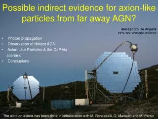
2. Motivation C. Burrage, A. Davis & D. Shaw, PRL 102 201101 (2009) recently introduced a new method for searching for axion-like particles and applied it to real AGN data, finding‘evidence strongly suggestive of the existence of a very light ALP.’ In a subsequent analysis, they raised the evidence of this claim to the 5 sigma level, though they acknowledge that there may be another explanation. Our analysis: Guido W. Pettinari & RC, arXiv:1007.0024

3. Scalar field couplings Cosmologists use scalar fields to solve a range of problems: • Initial conditions -- Inflaton • Dark Matter -- E.g. Axions • Late acceleration -- Quintessence field Aside from reheating, we usually ignore the couplings that these fields will have to ordinary particles; this is because if such couplings were strong the fields would either not be dark, or would not cause acceleration. But such couplings, if not forbidden by some symmetry, are expected to exist, and they can lead to interesting phenomenology: • Time/space dependent couplings (e.g. fine structure constant) • Tired light models • Fifth force constraints E.g. Carroll (1998), Csaki et al (2002), Bassett & Kunz (2004), etc.

4. Axions and the like The axion is pseudo Nambu-Goldstone boson invented to solve the strong CP problem. It is a potential candidate for dark matter. It has a coupling to photons of the form: The coupling is constrained in many ways: • Solar energy loss • Direct searches for solar axions • Conversion to photons from SN1987A • Searches assuming it is dark matter Scalar particles can have similar interactions and these are even more constrained by fifth force tests. Generically particles with such couplings will be called axion-like particles (ALPs). Scalar coupling Pseudo-scalar coupling

5. Chameleon fields Most of the constraints on ALPs can be avoided if the fields are chameleon-like, with masses which depend on the local density. Kouray & Weltman PRD 69 044026 (2004) Where and the potential takes a particular form. This interaction arises when the scalar field is non-minimally coupled to gravity and you transform to a frame where the gravity is simple. The impact of the interaction is that the evolution depends on the local matter density: Limits made in high density environments no longer apply!

6. Mixing and magnetic fields Thus, its interesting to try to constrain ALPs where the interaction is in low density environments. One possibility is looking at photons travelling through cluster magnetic fields, converting into axions. The probability of this is: Here, and For a cluster magnetic field, B ~ 1-10 mG and Lcoh ~ 1-100 kpc. In the strong mixing limit the mixing becomes energy independent at high energies, This can also happen if the photons pass through N independent domains, as long as NP > 1. Strong mixing occurs when E > 0.3-3 keV for typical parameters.

7. Cartoon picture Light from distant sources passes through cluster magnetic fields, and the more energetic photons experience strong mixing into axion-like particles, reducing the luminosity in photons. Hard photons Axions Soft photons Cluster magnetic field Quasar Less energetic light is not mixed, leaving it unaffected. The ratio of luminosities is reduced by 1/3 on average, but the precise amount varies depending on magnetic field strength and orientation on the LOS.

8. Resulting distribution Assuming that strong mixing occurs, the final photon luminosity is suppressed by a factor which varies from one line of sight to another. The distribution of this suppression can be predicted given the degree of the initial polarization. Burrage, Davis and Shaw proposed to look for this characteristic distribution in the ratios of different energy photons. In the analysis that follows, the initial photon polarization has marginal impact, so I will ignore it. Distribution of ratios of final to initial intensity.

9. Intrinsic scatter There is not a one to one correspondence between high and low energy luminosities, as they may be emitted via different physical mechanisms. In the absence of a full underlying model, the relationship is often modeled phenomenologically, Here, a and b describe the average calibration, which are derived from the data. S describes the scatter around this fit, which is often reasonably described by a Gaussian distribution. Here we focus on the scatter rather than the average behavior. Thus, the average 1/3 reduction in luminosity is absorbed in the calibration. However, the mixing provides an extra contribution to the scatter which is non-Gaussian and can be measured!

10. Predictions for the scatter Assuming the intrinsic scatter is Gaussian, we can predict the distribution for how the observed scatter should look after strong mixing: • The impact depends on two factors: • the degree of intrinsic scatter • the fraction of LOS to experience strong mixing – Pmix • Mixing increases the variance of the scatter by a fixed amount, and also adds to the low luminosity tail. Derived initially by Burrage, Davis & Shaw, 09.

11. Searching for the effect • To search for the effect, BDS analyzed a sample of 77 AGN with optical and X-ray luminosities. • They examined the ratio between the likelihoods for two hypotheses: • Assuming purely Gaussian scatter with the observed variance • Assuming intrinsic Gaussian scatter, folded with additional scatter from mixing, with the same total variance. • They found a statistic, which they called r, which is effectively the difference in chi-squared. • For their data set, they found r = 14, corresponding to 3.7 s evidence for the scattering model. • For a larger data set with 203 AGN, they found r = 25, or 5 s evidence for the scattering model!

12. Fingerprints of mixing • Another line of evidence that BDS cite is the distribution of variance and skewness in bootstrap re-samplings of the data set, compared to similar re-samplings of single realizations of Gaussian and ALP mixing. • The data resemble the ALP realization much more closely than the Gaussian one, though BDS do not try to quantify it. • Two significant similarities: • Large skewness when variance is large. • Similar substructure seen which is not present in Gaussian bootstraps. Combined with the r-statistic, these seem to make a strong case for the axion mixing model.

13. What’s going on? Where is the substructure coming from? We reproduced their results, but found the substructure only arose in simulations where there were large outliers. One or two outliers are being re-sampled, and re-sampling them more than once increases the variance and skewness, and so creates a new substructure. The substructure occurs in mixing simulations, but it is not typical. These fingerprints show that the data has one or two outliers which are skewed to lower luminosity.

14. The cumulative distribution These outliers can be clearly seen in the CDF. One or two outliers dominate the tail of the distribution. Notably, the mixing model is more likely to have these outliers because it has a wider tail and is skewed in the same way as the data. However, the outliers exceed what is expected in the ALP model. While mixing is a much better fit than Gaussian, neither really works. These outliers dominate both the ratio of likelihoods and the fingerprint plots. Removing the biggest outlier reduces the r statistic by 64% in the BDS data set! This object is known to be highly obscured in the X-ray with strong absorption features.

15. What should we have seen? The measured r value of 14 is in fact much higher than what is predicted in the ALP mixing model. By Monte Carlo-ing many samples of the model, we find that typically we should not have expected a significant signal with the data set used by BSD. To get a significant signal, one needs either many more AGN, or a sample with a smaller intrinsic variance, so that the effects of mixing are more obvious.

16. A new sample • Motivated by these issues, we analyzed a new data set based on SDSS and the XMM-Newton quasar survey (M. Young et al, 2009.) • Advantages of the new survey: • Homogeneous X-ray observations • Multiple x-ray bands (1, 1.5, 2, 4, 7, 10 keV) • Many thousands of photons, so that photon shot noise is minimal • More objects • We attempt to make a homogeneous subsample of these, excluding any which: • Appear to be radio loud or broad line emission sources • Have a significant signal/noise (average 1300 photons) • X-ray spectra are not well fit by a power law • Spectral slope might indicate obscured AGN. • This results in a sample 320 AGN with relatively small variance.

17. Do we have the sensitivity? With this new sample, in principle we could find good evidence for mixing, if the probability of mixing is high enough: A four sigma detection is expected if the probability of mixing is 50% or higher.

18. Results Apart from the 1 keV bin (r = 9), which is most likely to still be affected by absorption, all the other X-ray bins actually prefer the Gaussian distribution. However, neither model gives great goodness of fit, as quantified by KS, Kuiper and Anderson-Darling tests. r = 9 r = -8

19. Conclusions • The distribution of the ratios of the high and low energy luminosities of objects can in principle give useful bounds on mixing to axion-like particles, but it requires a homogeneous class of objects where the intrinsic scatter is reasonably small and preferably is well understood. • Even a few objects could be enough if the scatter is small and we can be certain that they should have been strongly mixed by passing through magnetic field regions. • Early indications of evidence for such mixing are contaminated by inhomogeneous sources, and in particular by a few outliers where the X-rays have been strongly absorbed. • Analysis of more homogeneous samples shows no evidence, indicating either no mixing, or that the probability of mixing is less than 50%.