Download
1 / 29
320 likes | 663 Views
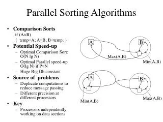
Parallel Sorting Algorithms. Potential Speedup. O( n log n ) optimal sequential sorting algorithm Best we can expect based upon a sequential sorting algorithm using n processors is:. Compare-and-Exchange Sorting Algorithms.

E N D
Potential Speedup O(nlogn) optimal sequential sorting algorithm Best we can expect based upon a sequential sorting algorithm using n processors is:
Compare-and-Exchange Sorting Algorithms Form the basis of several, if not most, classical sequential sorting algorithms. Two numbers, say A and B, are compared between P0 and P1. P0 P1 A B MIN MAX
Odd-Even Transposition Sort - example Parallel time complexity: Tpar = O(n) (for P=n)
Odd-Even Transposition Sort – Example (N >> P) Each PE gets n/p numbers. First, PEs sort n/p locally, then they run odd-even trans. algorithm each time doing a merge-split for 2n/p numbers. P0 P1 P2 P3 13 7 12 8 5 4 6 1 3 9 2 10 Local sort 7 12 13 4 5 8 1 3 6 2 9 10 O-E 4 5 7 8 12 13 1 2 3 6 9 10 E-O 4 5 7 1 2 3 8 12 13 6 9 10 O-E 1 2 3 4 5 7 6 8 9 10 12 13 E-O SORTED:1 2 3 4 5 6 7 8 9 10 12 13 Time complexity:Tpar = (Local Sort) + (p merge-splits) +(p exchanges) Tpar = (n/p)log(n/p) + p*(n/p) + p*(n/p) = (n/p)log(n/p) + 2n
BitonicMergesort Bitonic Sequence A bitonic sequenceis defined as a list with no more than one LOCAL MAXIMUM and no more than one LOCAL MINIMUM. (Endpoints must be considered - wraparound )
A bitonic sequenceis a list with no more than one LOCAL MAXIMUM and no more than one LOCAL MINIMUM. (Endpoints must be considered - wraparound ) This is ok! 1 Local MAX; 1 Local MIN The list is bitonic! This is NOTbitonic! Why? 1 Local MAX; 2 Local MINs
Binary Split • Divide the bitonic list into two equal halves. • Compare-Exchange each item on the first half • with the corresponding item in the second half. Result: Two bitonic sequences where the numbers in one sequence are all less than the numbers in the other sequence.
Repeated application of binary split Bitonic list: 24 20 15 9 4 2 5 8 | 10 11 12 13 22 30 32 45 Result after Binary-split: 10 11 12 9 4 2 5 8 | 24 20 15 13 22 30 32 45 If you keep applying the BINARY-SPLIT to each half repeatedly, you will get a SORTED LIST ! 10 11 12 9 . 4 2 5 8 | 24 20 15 13 . 22 30 32 45 4 2 . 5 8 10 11 . 12 9 | 22 20 . 15 13 24 30 . 32 45 4 . 2 5 . 8 10 . 9 12 .11 15 . 13 22 . 20 24 . 30 32 . 45 2 4 5 8 9 10 11 12 13 15 20 22 24 30 32 45 Q: How many parallel steps does it take to sort ? A: log n
Sorting a bitonic sequence Compare-and-exchange moves smaller numbers of each pair to left and larger numbers of pair to right. Given a bitonic sequence, recursively performing ‘binary split’ will sort the list.
Sorting an arbitrary sequence To sort an unordered sequence, sequences are merged into larger bitonic sequences, starting with pairs of adjacent numbers. By a compare-and-exchange operation, pairs of adjacent numbers formed into increasing sequences and decreasing sequences. Pairs form a bitonic sequence of twice the size of each original sequences. By repeating this process, bitonic sequences of larger and larger lengths obtained. In the final step, a single bitonic sequence sorted into a single increasing sequence.
Bitonic Sort Step No. 1 2 3 4 5 6 Processor No. 000 001 010 011 100 101 110 111 L H H L L H H L L L H H H H L L L H L H H L H L L L L L H H H H L L H H L L H H L H L H L H L H Figure 2: Six phases of Bitonic Sort on a hypercube of dimension 3
Bitonic sort (for N = P) P0 P1 P2 P3 P4 P5 P6 P7 000 001 010 011 100 101 110 111 K G J M C A N F Lo Hi Hi Lo Lo Hi High Low G K M J A C N F L L H HHH L L G J M K N F A C L H L H H L H L G J K M N F C A L LLL H HH H G F C A N J K M L L H H L L H H C A G F K J N M A C F G J K M N
Number of steps (P=n) In general, with n = 2k, there are k phases, each of 1, 2, 3, …, k steps. Hence the total number of steps is:
Bitonicsort (for N >> P) x xxx x xxx x xxx x xxx x xxx x xxx x xxx x xxx
Bitonic sort (for N >> P) P0 P1 P2 P3 P4 P5 P6 P7 000 001 010 011 100 101 110 111 2 7 4 13 6 9 4 18 5 12 1 7 6 3 14 11 6 8 4 10 5 2 15 17 Local Sort (ascending): 2 4 7 6 9 13 4 5 18 1 7 12 3 6 14 6 8 11 4 5 10 2 15 17 L H H L L H High Low 2 4 6 7 9 13 7 12 18 1 4 5 3 6 6 8 11 14 10 15 17 2 4 5 L L H HHH L L 2 4 6 1 4 5 7 12 18 7 9 13 10 15 17 8 11 14 3 6 6 2 4 5 L H L H H L H L 1 2 4 4 5 6 7 7 9 12 13 18 14 15 17 8 10 11 5 6 6 2 3 4 L LLL H HHH 1 2 4 4 5 6 5 6 6 2 3 4 14 15 17 8 10 11 7 7 9 12 13 18 L L H H L L H H 1 2 4 2 3 4 5 6 6 4 5 6 7 7 9 8 10 11 14 15 17 12 13 18 L H L H L H L H 1 2 2 3 4 4 4 5 5 6 6 6 7 7 8 9 10 11 12 13 14 15 17 18
Parallel sorting - summary • Computational time complexity using P=n processors • Odd-even transposition sort - O(n) • Parallel mergesort - O(n) • unbalanced processor load and Communication • BitonicMergesort - O(log2n) (** BEST! **) • ??? Parallel Shearsort- O(n logn) (* covered later *) • Parallel Rank sort - O(n) (for P=n) (* covered later *)
Sorting on Specific Networks • Two network structures have received special attention: • meshand hypercube • Parallel computers have been built with these networks. • However, it is of less interest nowadays because networks got faster and clusters became a viable option. • Besides, network architecture is often hidden from the user. • MPI provides libraries for mapping algorithms onto meshes, and one can always use a mesh or hypercube algorithm even if the underlying architecture is not one of them.
Two-Dimensional Sorting on a Mesh The layout of a sorted sequence on a mesh could be row by row or snakelike:
Shearsort Alternate row and column sorting until list is fully sorted. Alternate row directions to get snake-like sorting:
Shearsort – Time complexity On a n x n Mesh, it takes 2log n phases to sort n2 numbers. Therefore: Since sorting n2 numbers sequentially takes Tseq = O(n2 log n);
Rank Sort • Number of elements that are smaller than each selectedelement is counted. This count provides the position of the selected number, its “rank” in the sorted list. • First a[0] is read and compared with each of the other numbers, a[1] … a[n-1], recording the number of elements less than a[0]. • Suppose this number is x. This is the index of a[0] in the final sorted list. • The number a[0] is copied into the final sorted list b[0] … b[n-1], at location b[x]. Actions repeated with the other numbers. • Overall sequential time complexity of rank sort: Tseq = O(n2) • (not a good sequential sorting algorithm!)
Sequential code for (i = 0; i < n; i++) { /* for each number */ x = 0; for (j = 0; j < n; j++) /* count number less than it */ if (a[i] > a[j]) x++; b[x] = a[i]; /* copy number into correct place */ } *This code needs to be fixed if duplicates exist in the sequence. sequential time complexity of rank sort: Tseq = O(n2)
Parallel Rank Sort (P=n) One number is assigned to each processor. Pi finds the final index of a[i] in O(n) steps. forall (i = 0; i < n; i++) { /* for each no. in parallel*/ x = 0; for (j = 0; j < n; j++) /* count number less than it */ if (a[i] > a[j]) x++; b[x] = a[i]; /* copy no. into correct place */ } Parallel time complexity, O(n), as good as any sorting algorithm so far. Can do even better if we have more processors. Parallel time complexity: Tpar = O(n) (for P=n)
Parallel Rank Sort with P = n2 Use n processors to find the rank of one element. The final count, i.e. rank of a[i] can be obtained using a binary addition operation (global sum MPI_Reduce()) Time complexity (for P=n2): Tpar = O(log n) Can we do it in O(1) ?