Lecture 12: Generalized Linear Models (GLM)
Lecture 12: Generalized Linear Models (GLM). What are they? When do we use it? The full model The ANCOVA model The common regression model The extra sum of squares principle Assumptions. What are General(ized) Linear Models. Multivariate models. GLMs are models of the form:

Lecture 12: Generalized Linear Models (GLM)
E N D
Presentation Transcript
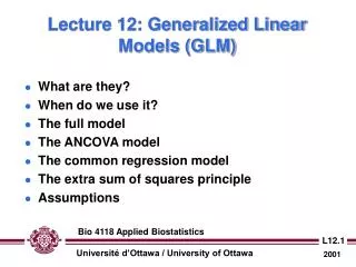
Lecture 12: Generalized Linear Models (GLM) • What are they? • When do we use it? • The full model • The ANCOVA model • The common regression model • The extra sum of squares principle • Assumptions Bio 4118 Applied Biostatistics
What are General(ized) Linear Models Multivariate models • GLMs are models of the form: • with Y, a vector of dependent variables, b, a vector of estimated coefficients, X, a vector of independent variables and e, a vector of error terms. Simple linear regression Multiple regression Analysis of variance (ANOVA) Analysis of covariance (ANCOVA) Bio 4118 Applied Biostatistics
Some GLM procedures *either categorical or treated as a categorical variable Bio 4118 Applied Biostatistics
Body size Body mass Body size When do we use ANCOVA? • to compare the relationship between a dependent (Y) and independent (X1) variable for different levels of one or more categorical variables (X2) • e.g. relationship between body mass (Y) and body size (X1) for different taxonomic groups (birds & mammals, X2) Bio 4118 Applied Biostatistics
Y Qualitatively similar models Y Qualitatively different models Level 1 of X2 Level 2 of X2 X1 When do we use ANCOVA? • In doing comparisons, we assume that the qualitative form of the model is the same for all levels of the categorical variables... • …otherwise, one is comparing apples and oranges! Bio 4118 Applied Biostatistics
Y Linear models X1 Y Non- linear models Level 1 of X2 Level 2 of X2 X1 When do we use ANCOVA? • ANCOVA is used to compare linear models … • … although ANCOVA-like extensions have been developed for nonlinear models. Bio 4118 Applied Biostatistics
ei Yi DY Xi DX X Observed Expected The simple regression model • The regression model is: • So, all simple regression models are described by 2 parameters, the intercept (a) and slope (b). a (intercept) b = DY/DX (slope) Bio 4118 Applied Biostatistics
Y Different a & b X1 Y Different a, sameb X1 Simple GLMs • Two linear models may differ as follows: • differences in both intercepts (a) and slopes (b) • different intercepts but the same slopes (ANCOVA model) Bio 4118 Applied Biostatistics
Y Same a, different b X1 Y Same a, sameb X1 Simple GLMs • Two linear models may also differ as follows: • different slopes (b) but the same intercepts (a) • same slopes and intercepts (common regression model) Bio 4118 Applied Biostatistics
Fitting GLMs Model A (term in) • Proceeds in hierarchical fashion fitting the most complex model first. • Evaluate significance of a term by fitting two models: one with the term in, the other with it removed. • Test for change in model fit (D MF) associated with removal of the term in question. D MF Model B (term out) Retain term (D large) Delete term (D small) Bio 4118 Applied Biostatistics
Model fitting: evaluating the significance of model terms Higher order model • Fit higher order model (hom) including all possible terms; retain SSresidualand MSresidual . • Fit reduced model (rm), retain SSresidual . • Test for significance of removed term by computing: F Reduced model Retain term (p < .05) Delete term (p > .05) Bio 4118 Applied Biostatistics
m Level 1 of variable X2 Level 2 of variable X2 The full model with 2 independent variables • The full model is: • bi is the slope of the regression of Y on X1 (the covariate) estimated for level i of the categorical variable X2 . • ai is the difference between the mean of each level i of the categorical variable X2 and the overall mean. Bio 4118 Applied Biostatistics
m Level 1 of variable X2 Level 2 of variable X2 The full model : null hypotheses • For the full model with 2 independent variables, there are 3 null hypotheses: Bio 4118 Applied Biostatistics
Y Y Y Bio 4118 Applied Biostatistics
Assumptions for full model hypothesis testing • Residuals are independent and normally distributed. • Residual variance is equal for all values of X and independent of the value of the categorical variable (homoscedasticity). • No error in independent variables • Relationship between Y and covariate is linear. Bio 4118 Applied Biostatistics
Y X1 ANCOVA Separate regressions Procedure • Fit full model, test for differences among slopes. • If H02 rejected, run separate regressions for each level of categorical variable(s). • If H02 accepted, proceed to fit ANCOVA model. H02 accepted H02 rejected Level 1 of variable X2 Level 2 of variable X2 Bio 4118 Applied Biostatistics
m Level 1 of variable X2 Level 2 of variable X2 The ANCOVA model with 2 independent variables • The full model is: • b is the slope of the regression of Y on X1 (the covariate)pooled over levels of the categorical variable X2 . • ai is the difference between the mean of each level i of the categorical variable X2 and the overall mean. Bio 4118 Applied Biostatistics
m Level 1 of variable X2 Level 2 of variable X2 The ANCOVA model: null hypotheses • For the ANCOVA model with 2 independent variables, there are 2 null hypotheses: Bio 4118 Applied Biostatistics
Y Y Y Bio 4118 Applied Biostatistics
Assumptions for hypothesis testing in ANCOVA model • Residuals are independent and normally distributed. • Residual variance is equal for all values of X and independent of the value of the categorical variable (homoscedasticity). • No error in independent variables • Relationship between Y and covariate is linear. • The slope of the regression of Y on X1 (the covariate) is the same for all levels of the categorical variable X2 (not an assumption for full model!). Bio 4118 Applied Biostatistics
Y X1 Common regression Multiple comparisons Procedure • Fit ANCOVA model; test for differences among intercepts. • If H01 rejected, do multiple comparisons to see which intercepts differ (if there are more than 2 levels for X2). • If H01 accepted, proceed to fit common regression model. H01 accepted H01 rejected Level 1 of variable X2 Level 2 of variable X2 Bio 4118 Applied Biostatistics
a Level 1 of variable X2 Level 2 of variable X2 The common regression model with 2 independent variables • The model is: • b is the slope of the regression of Y on X1pooled over levels of the categorical variable X2 . • ais the pooled intercept. • is the pooled average of X1. Bio 4118 Applied Biostatistics
a Level 1 of variable X2 Level 2 of variable X2 The common regression model : null hypotheses • For the common regression model, there are 2 null hypotheses: Bio 4118 Applied Biostatistics
Assumptions for hypothesis testing in common regression model • Residuals are independent and normally distributed. • Residual variance is equal for all values of X. • No error in independent variable • Relationship between Y and X is linear. Bio 4118 Applied Biostatistics
Example 1: effects of sex and age on sturgeon size at The Pas Females Males Bio 4118 Applied Biostatistics
Analysis Males • Log(forklength)(LFKL) is dependent variable; log(age) (LAGE) is the covariate, and sex (SEX$) is the categorical variable (2 levels). • Q1: is slope of regression of LFKL on LAGE the same for both sexes? Females Bio 4118 Applied Biostatistics
Effects of sex and age on size of sturgeon at The Pas Bio 4118 Applied Biostatistics
Analysis Males • Conclusion 1: slope of regression of LFKL on LAGE is the same for both sexes (accept H03) since p(SEX$*LAGE) > .05 . • Q2: is intercept the same for both males and females? Females Bio 4118 Applied Biostatistics
Effects of sex and age on size of sturgeon at The Pas (ANCOVA model) Bio 4118 Applied Biostatistics
Analysis Males • Conclusion 2: Intercept is the same for both males and females. H02 is accepted since p(SEX$ > 0.05), implying that… • …best model is common regression model. • Note that reduction in fit (R2) from full model to ANCOVA model is negligible (.697 to .696) indicating that deleting a model term has a negligible impact on model fit. Females Bio 4118 Applied Biostatistics
Effects of sex and age on size of sturgeon at The Pas (common regression) Bio 4118 Applied Biostatistics
Example 2: Effect of location and age on sturgeon size LFKL LFKL Bio 4118 Applied Biostatistics
1.9 1.8 LFKL 1.7 1.6 1.5 1.0 1.1 1.2 1.3 1.4 1.5 1.6 1.7 1.8 LAGE Analysis Lake of the Woods • Log(forklength)(LFKL) is dependent variable; log(age) (LAGE)is the covariate, and location (SEX$) is the categorical variable (2 levels). • Q: is slope of regression of LFKL on LAGE the same at both locations? Nelson River LFKL Bio 4118 Applied Biostatistics
Effect of location and age on sturgeon size Bio 4118 Applied Biostatistics
Analysis Lake of the Woods LFKL • Conclusion: slope of regression of LFKL on LAGE is different at the two locations (reject H03) since p(LOCATION$*LAGE) < .05 . • So, should fit individual regressions for each location. Nelson River LFKL Bio 4118 Applied Biostatistics
More than 2 levels of categorical variable? Follow above procedure but if H03(same slope) rejected, do pairwise contrasts of individual slopes. If H03 accepted but H02(same intercepts) rejected, do pairwise comparisons of intercepts. Always control for experiment-wise Type I error rate. Y X What do you do if? Bio 4118 Applied Biostatistics
Biological hypothesis implies one-tailed null(s)? Follow above procedure but if H03(same slope) rejected, do one-tailed pairwise contrasts of individual slopes. If H03 accepted but H02(same intercepts) rejected, do one-tailed pairwise comparisons of intercepts. Y X What do you do if? Bio 4118 Applied Biostatistics
Power analysis in GLM • In any GLM, hypotheses are tested by means of an F-test. • Remember: the appropriate SSerror and dferrordepends on the type of analysis and the hypothesis under investigation. • Knowing F,we can compute R2,the proportion of the total variance in Y explained by the factor (source) under consideration. Bio 4118 Applied Biostatistics
Partial and total R2 Proportion of variance accounted for by both A and B (R2Y•A,B) • The totalR2 (R2Y•B) is the proportion of variance in Y accounted for (explained by) a set of independent variables B. • The partialR2 (R2Y•A,B- R2Y•A ) is the proportion of variance in Y accounted for by B when the variance accounted for by another set A is removed. Proportion of variance accounted for by B independent of A (R2Y•A,B- R2Y•A ) (partial R2) Proportion of variance accounted for by A only (R2Y•A)(total R2) Bio 4118 Applied Biostatistics
Y A A B Partial and total R2 Proportion of variance independent of A (R2Y•A,B- R2Y•A ) (partial R2) Proportion of variance accounted for by B (R2Y•B)(total R2) • The totalR2 (R2Y•B) for set B equals the partialR2 (R2Y•A,B- R2Y•A ) for set B if either (1) the total R2 for A (R2Y•A) is zero; or (2) if A and B are independent (in which case R2Y•A,B= R2Y•A + R2Y•B). Equal iff Bio 4118 Applied Biostatistics
Y X 0.20 0.16 0.12 Growth rate l (cm/day) 0.08 0.04 0.00 28 20 24 16 Water temperature (°C) Partial and total R2 • In simple linear regression and single-factor ANOVA, there is only one independent variable X (either continuous or categorical). • In these cases, set B includes only one variable X andtotalR2 (R2Y•B) = totalR2 (R2Y•X) and the partial and total R2 are the same. Bio 4118 Applied Biostatistics
Y X1 0.20 0.16 0.12 Growth rate l (cm/day) 0.08 0.04 16 20 24 28 0.00 pH = 6.5 pH = 4.5 Water temperature (°C) Partial and total R2 • In ANCOVA and multiple-factor ANOVA, there are several independent variables X1, X2, ... (either continuous or categorical), so set B includes several variables. • In this case, the total and partial R2 may be very different. Bio 4118 Applied Biostatistics
Y X2 = L1 X2 = L2 X1 Example: Partial and total R2 in ANCOVA • Two independent variables: X1 (continuous) and X2 (categorical) Bio 4118 Applied Biostatistics
Defining effect size in GLM • The effect size, denoted f2, is given by the ratio of the factor (source) R2factor and 1 minus the appropriate error R2error. • Note: both R2factor and R2error depend on the null hypothesis under investigation. Bio 4118 Applied Biostatistics
Effects of sex and age on size of sturgeon at The Pas (common regression) Bio 4118 Applied Biostatistics
Case 1: a set B is related to Y, and the totalR2 (R2Y•B) is determined. The error variance proportion is then 1- R2Y•B . H0: R2Y•B = 0 Example: effect of age on sturgeon size at The Pas B = {LAGE} Defining effect size in GLM: case 1 Bio 4118 Applied Biostatistics
Effects of sex and age on size of sturgeon at The Pas Bio 4118 Applied Biostatistics
Effects of sex and age on size of sturgeon at The Pas (ANCOVA model) Bio 4118 Applied Biostatistics
Case 2: the proportion of variance of Y due to B over and above that due to A is determined (R2Y•A,B- R2Y•A ). The error variance proportion is then 1- R2Y•A,B . H0: R2Y•A,B- R2Y•A = 0 Example: effect of SEX$*LAGE on sturgeon size at The Pas B ={SEX$*LAGE}, A,B = {SEX$, LAGE, SEX$*LAGE} Defining effect size in GLM: case 2 Bio 4118 Applied Biostatistics
Once f2 has been determined, either a priori (as an alternate hypothesis) or a posteriori (the observed effect size), calculate non-central F parameter f . Knowing f and factor (source) (n1) and error (n2) degrees of freedom, we can determine power from appropriate tables for given a. Decreasing n2 n1 = 2 1-b a = .05 a = .01 f(a = .05) 2 4 5 3 f(a = .01) 1 1.5 2 2.5 Determining power Bio 4118 Applied Biostatistics