Download
1 / 61
610 likes | 775 Views
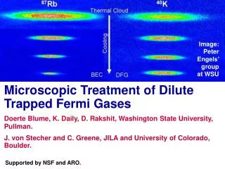
Image: Peter Engels’ group at WSU. Microscopic Treatment of Dilute Trapped Fermi Gases. Doerte Blume, K. Daily, D. Rakshit, Washington State University, Pullman. J. von Stecher and C. Greene, JILA and University of Colorado, Boulder. Supported by NSF and ARO. Introduction:

E N D
Image: Peter Engels’ group at WSU Microscopic Treatment of Dilute Trapped Fermi Gases Doerte Blume, K. Daily, D. Rakshit, Washington State University, Pullman. J. von Stecher and C. Greene, JILA and University of Colorado, Boulder. Supported by NSF and ARO.
Introduction: BCS-BEC (Bardeen-Cooper-Schrieffer) crossover (s-wave interacting “up” and “down” atoms with equal masses and no population-imbalance). Theoretical challenges. A few examples of our trapped few-fermion studies: Universality throughout crossover and at unitarity. Natural orbitals, occupation numbers and momentum distribution. [Not today: Highly-polarized system, unequal masses, trap-imbalanced, effectively low-dimensional, p-wave.] Summary Outline of This Talk
BCS-BEC Crossover with Cold Two-Component Atomic Fermi Gas Normalized energy crossover curve N “BCS” Weakly-repulsive molecular Bose gas Weakly-attractive atomic Fermi gas 1h “BEC” aho/as Strongly- interacting (unitarity) STABLE GAS!!! Images (experiment): Jin group, JILA.
“Up” - “Down” Interactions: Two-Body s-Wave Scattering Length At low temperature, the details of the atom-atom potential are irrelevant: Positive s-wave scattering length: Effective repulsive interaction. Negative s-wave scattering length: Effective attractive interaction. weakly- interacting (attraction) weakly- interacting (repulsion) as as strongly- interacting BEC- SIDE BCS- SIDE Dilute gas: r0 << aho, as or n(0)r03 << 1. as Similarities with nuclear matter, condensed matter/ Cooper pairs. Ebind external control parameter (B-field)
Microscopic to macroscopic: Other examples: Doped helium clusters: Molecular rotations, microscopic superfluidity,... Metal clusters: conductivity, designing materials,... What is special about dilute atomic Fermi systems? Controllable system (scattering length, trap geometry,…) Universal behavior. Our General Philosophy: From Few to Many atomic/ molecular condensed matter ? “mesoscopic” External confining potential optical lattice
Three motivations: Few-body physics is interesting and determines some properties of the many-body system. Commonalities of few- and many-body system. Benchmark of theoretical techniques. Challenge: Naïve computational approaches scale exponentially with number of degrees. Possible solutions: Introduce stochastic element (Monte Carlo) Use “smart” basis: Microscopic Theoretical Description r0 aho r
Virial Expansion for Fermi Gas Based on Two- and Three-Fermion Spectra Complete N=3 spectrum (calculated following Kestner and Duan, PRA 76, 033611 (2007)): “High-T” thermodynamics in trap (virial coefficients calculated from two- and three-body energies): L=0 L=1 Liu et al., PRL 102, 160401 (2009)
Up to N=7: Basis set expansion (CG) approach. Use Gaussian two-body potential and correlated Gaussian basis functions (plus generalized spherical harmonic): = Np |v|L YLM(v) exp(-xTAx) x collectively denotes N-1 Jacobi coordinates. v = ux A denotes (N-1)x(N-1) dimensional parameter matrix. u denotes N-1 dimensional parameter vector. Hamiltonian matrix can be evaluated analytically. Rigorous upper bound (“controlled accuracy”). Computational effort increases with N: Evaluation of Hamiltonian matrix elements involves diagonalizing (N-1)x(N-1) matrix. Permutations Np scale nonlinearly (Np=2,4,12,36,144 for N=3,4,5,6,7). How Do We Solve Stationary Many-Body Schrödinger Equation? CG. H = i (Ti + Vtrap,i) + I<j Vtwobody,ij For details see: Suzuki and Varga; von Stecher, Greene, Blume, PRA 77, 043619 (2008).
Up to N=30: Fixed-node diffusion Monte Carlo (FN-DMC) approach. Fermionic symmetry imposed by nodal structure of so-called guiding function T (input): Nodal surface coincides with that of non-interacting Fermi gas: T det()det() (homogeneous system: “normal”). Nodal surface determined by two-body solution (rii’): T A((1,1’),…, (N/2,N/2’)) (homogeneous system: “superfluid”). Rigorous upper bound for energy of state that has the same symmetry as T. Structural properties may “suffer” some bias (hopefully negligible). Stochastic method: Observables have (controllable) error bar. Up to N=7: Comparison between CG and FN-DMC results. How Do We Solve Stationary Many-Body Schrödinger Equation? FN-DMC. H = i (Ti + Vtrap,i) + I<j Vtwobody,ij For details see: von Stecher, Greene, Blume, PRA 77, 043619 (2008).
Absence of many-body bound state if no (s-wave scattering length as<0) / one (as>0) two-body bound state exists: 2 up and 2 down with zero-range interactions: Petrov et al. Holds also for small systems with finite range interactions (at least for the interactions we looked at). Technical implication: State of interest = true ground state. Physical implication: Stability (Fermi pressure “counteracts” attractive interactions). In contrast, three- or many-body bound states exist for unequal mass Fermi systems, for Bose systems, and for three-component systems: leads, e.g., to Efimov physics. Our goal: Bottom-up study of 3D two-component Fermi system with equal masses under spherically harmonic confinement interacting through short-range s-wave interactions. Specifics for Small Equal-Mass Two-Component Fermi Systems
“Exact” CG calculations for simple model potentials. Benchmark for approximate numerical and analytical approaches: Monte Carlo (see later). Effective low-energy theories: Four-body problem is becoming tractable (Stetcu et al., PRA 76, 063613 (2007); Alhassid et al., PRL 100, 230401 (2008); Hammer et al.). Next: Unitarity and universality of crossover curves. Energy Crossover Curves for “Large” Few-Fermion Systems L=2 L=0 [E3D(4)-2E3D(2)] N=4 L=0 L=2 L=1 N=5
Unitarity: Only Relevant Length Scale is Oscillator Length Unitarity = Infinite scattering length E.g., N=5 (N=3, N=2), L=0: For zero-range interactions, “universal states” have been predicted to have peculiar properties [e.g., Werner et al., PRA 74, 053604 (2006)]: Excitation frequencies: 2nh. Hyperangular and hyperradial degrees of freedom separate. Solid lines: fit Energy minus 2h of third lowest L=0 state Symbols: CG (upper bound) Energy of lowest L=0 state Zero-range limit
Adiabatic relation: E/as = h2/(16 3mas2) C, where C denotes “integrated contact intensity”. Virial theorem: E = 2 <Vtrap> - h2/(323mas) C. Test of prediction: Use adiabatic relation as working definition of “contact” C and show that energy can be predicted using virial theorem. For us, practical test involves: Extrapolate finite range energies to zero range. Use ZR energies to obtain C using adiabatic relation. Compare energy calculated via virial theorem with extrapolated energy. Universality throughout Crossover for Zero Range Interactions Ho, Thomas, Tan, Werner, Castin, Braaten, Petrov,…
Evirial = 2<Vtrap> - as Eexact/as /2 - r0 Eexact/r0 /2 One Step Further: Include Finite Range Corrections Werner, PRA 78, 025601 (2008) “C(r0)” N=2, N=2 (L=0): Eexact-Evirial r0=0.01, 0.03, 0.05aho ZR Eexact-Evirial(as only) r0=0.05aho Generalized virial theorem validated on BCS side for N=4. Analysis is simplified by the fact that E depends linearly on r0.
Larger Trapped Two-Component Fermi Systems at Unitarity Zero scattering length: What happens to shell structure at unitarity (N-N=0,1)? Connection between energies of inhomogeneous and those of homogeneous system? Eunit=homENI; hom=0.42 Determination of excitation gap? Shell closure 20 8 Carlson et al., PRL (2003), Astrakharchik et al., PRL (2004)) 2
N1N20,1: Energy of Trapped Two-Component Fermi Gas at Unitarity Blume, von Stecher, Greene, PRL 99, 233201 (2007). smooth Monte Carlo energies: Local density approximation (even N): N1N21 (N odd) N1N20 (N even) We find: tr=0.467. For comparison: hom=0.42 (Carlson et al., PRL (2003), Astrakharchik et al., PRL (2004)) Even-odd oscillations. Essentially no shell structure.
Excitation Gap and Residual Oscillations at Unitarity See also, Chang and Bertsch, PRA 76, 021603(R ) (2007). N odd, N=N1+N2 and N1=N2+1 EFN-DMC-Efit (N) N1N21 DFT, Bulgac (PRA 76, 040502(R ), 2007) N1N20 residual oscillations
Local Density Approximation (LDA) not Valid for Odd-N system Spare particle sees local chemical potential: ( r)= 0 - V( r) for n( r)>0. Energy cost of introducing spare particle is ( r) plus ( r). Smallest near edge of cloud, where LDA breaks down. LDA: (N) N1/3 / We find trap=0.6. hom=0.85 (Carlson et. al. (2005)) (N) N1/9 (Son (2007)) also consistent with our data. FN-DMC (N)N1/3 DFT, Bulgac PRA (2007)
Beyond the Energy: Structural Properties at Unitarity Pair distribution function for up-down distance: Range r0=0.01aho. Very good agreement between CG and FN-DMC results. N=4: Enhanced probability at small r (pair formation). N=3 L=1 CG FN-DMC Positive scattering length N=4 L=0 Negative scattering length von Stecher, Greene, Blume, PRA 77, 043619 (2008).
One-body density matrix: (r’,r) =N …*(r’,r2,…,rN)(r,r2,…,rN)dr2…drN Decomposing (r’,r) = j nj j*(r)j(r’) with j*(r)j(r)dr = ij defines natural orbitals j(r) and occupation numbers nj. In practice, j(r) and nj are obtained by diagonalizing j*(r’)(r’,r)j(r)drdr’=nj. Alternatively, j(r) can be defined by writing (r’,r) = <+(r’)(r)>, where /+ are field operators that destroy/create a particle at position r, and by expanding (r)/+ (r) in terms of j(r)/j*(r) and aj/aj+ One-Body Density Matrix and Natural Orbitals
Occupation Numbers through Crossover: N=4 Natural orbitals depend on three coordinates: j(r) nl(r)Ylm(,) occupation of first l=0 natural orbital NI limit: l=0,2 nnlm/2 occupation of first l=1 natural orbital l=1 l=0
Little size dependence of “depletion”. In the near future: Two-body reduced density matrix pair fraction. Occupation Probability as Function of Number of Particles N=6 N=6 N=4 N=2 N=4
Momentum distribution can be written in terms of natural orbitals: n(k) = j nj|j(k)|2, where j(k) = (2)-3/2 exp(-ikr)(r)dr. It follows: n(k) = (2)-3 exp[ik(r-r’)](r’,r) drdr’. Partial wave decomposition: n(k) = lm nl(k) Ylm(k,k). Then: n(k)dk = (4)1/2 n0(k) Momentum Distribution for Trapped Two-Component Fermi System Shown on next slide for N=4
l=0 Projection of Momentum Distribution for N=4 2.5 5 7.5 10 aho/as=10 (4)-1/2 2.5 -2.5 unitarity NI
Cold atomic gases are nearly ideal systems for the experimental and theoretical study of few- and many-body physics. In particular, dilute atomic two-component Fermi gases are rich systems that have been and will continue to fascinate atomic, nuclear and condensed matter physicists: Universal energy crossover curves. Strongly-interacting regime / unitarity. Occupation numbers, momentum distribution,... Microscopic, few-particle studies provide perspective that complements condensed matter many-body approaches. Microscopic Treatment of Dilute Fermi Gases
Certain universal properties are independent of number of particles (unique energy level spacings, “universal parameter”,…). Certain many-body properties are determined by few-body physics (e.g., virial expansion [Liu et al., PRL 102, 160401 (2009)]). Some rigorous benchmark results can be obtained (may be more readily than for large systems, especially in strongly correlated regime). Experimental realization: Optical lattice with sufficiently deep and widely spaced lattice sites. Why Few-Fermion Systems? Interesting by Themselves… Bloch, Esslinger, Ketterle,… groups. optical lattice
Fast Rotating Fermi Gas: Effectively Two-Dimensional System z z z Fast rotation (~) No rotation N=3 (2D): No rotation N=3 (2D): Fast rotation Blume, unpublished.
Quasi-One-Dimensional System: Comparison of Full 3D and Strictly 1D N=3, Pz=1 Solutions are characterized by Pz and L: Here: L = 0. “BCS side”: 1D atomic Hamiltonian with renormalized atom-atom scattering length (Olshanii, PRL (1998)). “BEC side”: 1D molecular Hamiltonian: Molecules form in 3D and atom- dimer and dimer-dimer scattering lengths are renormalized. N=4, Pz=1 N=3, Pz=-1 Blume and Rakshit, arXiv:0901.3862v2
A Different Four-Body System: Four Identical Bosons D’Incao, von Stecher, Greene, arXiv:0903.3348 Four identical bosons: add aaa. Two up/two down fermions: add 0.6aaa.
Efimov effect/physics: Nuclear: 2n-rich halo nuclei, 12C Atomic: 4He trimer, Cs2+Cs, K2+K, three-body collisions. Three-component system: Nuclear: low density: nucleon = tri-quark bound state; high density: quark color superconductor. Atomic: Fermi gas with three internal states. Universal behavior (large scattering length as): Nuclear: neutron-neutron as = -18fm (effective range 2.8fm). Desirable: low density neutron matter. Atomic: Tunability of as near Feshbach resonance. Theoretical approaches… Where Do Atomic and Nuclear Physics Meet? Selected Examples. Experiment: Grimm, Inguscio groups. Experiment: Jochim, O’Hara groups. Experiment: Jin, Ketterle, Hulet, Thomas,… groups.
Energies for 2 and 3 Fermions in a Spherically Symmetric Harmonic Trap von Stecher, Greene, Blume, PRA 76, 053613 (2007); 77, 043619 (2008). Blume, unpublished. See also: Kestner and Duan, PRA 76, 033611 (2007); Stetcu et al., PRA 76, 063613 (2007). L=5 L=1 L=0 L=1 L=0 L=0 L=1 L=1 L=0
The Field of Cold Atom Physics EXPERIMENT THEORY Nobel Prizes: Laser cooling (1997): Chu, Cohen-Tannoudji, Phillips. Bose-Einstein condensation (2001): Cornell, Ketterle, Wieman. Theory of superconductors and superfluids (2003): Abrikosov, Ginzberg, Leggett. Quantum optics and frequency comb (2005): Glauber, Hall, Hänsch. nuclear physics molecular physics atomic physics condensed matter quantum information science quantum optics
4 Fermions = 2 Bosons: Dimer-Dimer Scattering Length and Effective Range von Stecher, Greene, Blume, PRA 76, 053613 (2007). First quantitative prediction for dimer-dimer effective range. 4 Fermions 2 Bosons Petrov et al., JPB 38, S645 (2005) FN-DMC CG Model dimer-dimer potential by zero-range interaction with energy-dependent dimer-dimer scattering length: rdd goes up as mass ratio increases: For =20, rdd~0.5add. Mass ratio
Excitation Gap at Unitarity for Equal-Mass Two-Component Fermi System See also, Chang and Bertsch, PRA 76, 021603(R ) (2007). N odd, N=N1+N2 and N1=N2+1 Local density approximation (LDA): (N) N1/3. But, LDA expected to break-down… Instead:(N) N1/9? (Son, arXiv:0707.1851) FN-DMC DFT, Bulgac PRA 76, 040502(R ) (2007)
Two-component Fermi gases with unequal masses, unequal trapping frequencies, unequal populations: Stability of unequal-mass systems (trimer formation)? Universal behavior? Phase separation? Multi-component s-wave interacting Fermi gas: Details of underlying two-body potential? Implications of existence or absence of three-particle negative energy states? Beyond s-wave: p-wave interactions? p-wave induced interactions? Related Topics and Natural Extensions
Interaction strengths can be controlled (Fano-Feshbach resonance). Confinement can be designed (lattice, quasi-1d,…). Fundamental physics question: Strongly-interacting system. Multi-component systems. Unequal mass systems. Efimov physics. Applications: High precision measurements of fundamental constants. Navigational devices. Quantum computation and quantum simulation. General Summary of Field of Cold Atom Physics
Look at Unitary Regime Differently: Hyperspherical Potential Curves h2CN/(2MR2) M2R2/2 Born-Oppenheimer like separation of variables: Divide coordinates into one hyperradius R and 3N-1 hyperangles. Integrate over angles, and analyze one-dimensional potential curve. At unitarity: V(R) = h2CN/(2MR2) + M2R2/2. Invert 1D SE to obtain CN. as=0 as= Werner et al., PRA 74, 053604 (2006) Rittenhouse et al. (2006) Even-odd oscillations evident in effective potential curves.
Comparison of Analytical and Numerical Hyperradial Wave Function CG FN-DMC N=15 N=4 (CG) N=9 N=6 N=4 (CG)
Graphics from JILA homepage. BCS BEC Weak attraction Weak repulsion
s-wave interaction strength of fermions can be tuned experimentally (Feshbach resonance). Smooth crossover for two-component system: Our study connects few- and many-body physics. Benchmark of nodal surface (input for FN-DMC calculations) for N=4 fermions. Crossover for multiple-component Fermi system appears to be not necessarily smooth (huge parameter space… strong dependence on range of two-body potential…). Next: p-wave interactions, anisotropic interactions,... Summary
Next: What happens if we implant impurity into BEC with repulsive atom-atom scattering length? Bound impurity state? Characteristics of Trapped Bose Gas: Stable versus Unstable 1 parameter Single particle orbital No solution to GP eq. Non-linearity BEC with attractive a, stabilized by trap BEC with repulsive scattering length a “snow- flake State” For 3-body treatment of collapse region, see Blume and Greene, PRA 66, 013601 (2002).
Treat trapped system: Determine free-space dimer-dimer scattering length and effective range from energies of trapped four-particle system. Weakly-interacting BEC and BCS limits: Determine validity regime of perturbative expressions. Universal properties of unitary gas: Intuitive ways to think about strongly-interacting system. Connect trapped system with homogeneous system: Validity of local density approximation? Gain better understanding of few- and many-body physics. Roadmap of Our Study of Two-Component Fermi Systems
Two-Fermion System with Mass- and Trap-Imbalance at Unitarity 1 6 2 4 Mass ratio=8 =1-(aho2/aho1)2 density density 2 decreases m2=8m1 m1=8m2 m1 m1 density x x m1=8m2 Equal frequencies m1 Blume, arXiv:0803.4221 x
Unitarity: What’s the Total Angular Momentum of Few-Body System? “BCS” Small N: Ltot=0 for even N and Ltot=1 for odd N Ltot=0 for even and odd N 1h ? “BEC” aho/as Ltot Symmetry inversion occurs on “BEC side” For N=3, see also Duan et al., PRA (2007) and van Kolck et al. (2007).
Crossover Curve for N=4: Different Mass Ratios, Equal Frequencies density FN-DMC (nodal surface of dimer pairs) m1=m2 FN-DMC (nodal surface of ideal gas) m2 x density m1=8m2 CG m2 x Size of non-interacting system: Next: Analyze molecular Bose gas.
Radial Density at Unitarity: Where Is “Spare” Atom Located? N=15 N=9 N=3 N=9: “Extra” particle more delocalized. N=15: “Extra” particle sits near the surface.
Coefficients of Hyperradial Potentials Obtained from FN-DMC Energies Odd N 0.42 Normalized coefficient Even N Turn-around of red curve? Problem with guiding function? Convergence for large N?
Experimental Signatures Bose Einstein Condensate of 87Rb (bosons): Macroscopic quantum object (“super-molecule”) Low T (a few nK) High T (Picture taken from JILA homepage) 40K (fermion) Looks just like the “ordinary” atomic condensate. Regal, Greiner, Jin, PRL 92, 040403 (2004)
Intuitive Way of Understanding Two-Body Scattering Length At low temperature, the details of the atom-atom potential are irrelevant: Positive scattering length: Effectively repulsive interaction. Negative scattering length: Effectively attractive interaction. Bosonic atoms in harmonic trap: N bosons in a box. Constant density. Periodic boundary conditions. BEC with attractive a, stabilized by trap Positive scattering length: Stable gas (not self-bound). Negative scattering length: Gas not stable; collapse toward solid or liquid (self-bound). BEC with repulsive scattering length a “snow- flake state”