Download
1 / 18

E N D
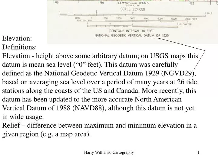
Elevation:Definitions: Elevation - height above some arbitrary datum; on USGS maps this datum is mean sea level (“0” feet). This datum was carefully defined as the National Geodetic Vertical Datum 1929 (NGVD29), based on averaging sea level over a period of many years at 26 tide stations along the coasts of the US and Canada. More recently, this datum has been updated to the more accurate North American Vertical Datum of 1988 (NAVD88), although this datum is not yet in wide usage.Relief – difference between maximum and minimum elevation in a given region (e.g. a map area). Harry Williams, Cartography
Past attempts to Portray Elevation on Maps: Pictorial representation Harry Williams, Cartography
Hachures Harry Williams, Cartography
Layer Shading Harry Williams, Cartography
Hill Shading Harry Williams, Cartography
Bench marks, spot heights and contours: Bench Marks: Harry Williams, Cartography
Bench marks are bronze disks, usually set in concrete. They are accurately surveyed geodetic control points. Traditionally, geodetic control is categorized as primary, secondary, or supplemental. Primary (First Order) control is used to establish geodetic points and to determine the size and shape of the earth. Secondary (Second Order) Class I control is used for network densification in urban areas and for precise engineering projects. Supplemental (Second Order, Class II and Third Order) control is used for network densification in non-urban areas and for surveying and mapping projects. Accuracy classifications such as these provide a common means to judge the quality of a point and its appropriateness for use in other work. Harry Williams, Cartography
Bench marks are shown on USGS maps by BM x 567 Example of Bench Mark Record: BENCH MARK DESCRIPTIONSAND ELEVATIONSBROWN COUNTY, INDIANA USGS BM TT 26 SC 1942 In Brown County, Elkinsville Quad, in the NW ¼ of Section 1, T. 7 N., R. 1 E., 2 nd P.M.; about 5.5 miles west of Elkinsville; at the Chambers Bridge over Middle Fork Salt Creek, at the “T” road intersection of Paynetown Road and Knightsridge Road; set in the top of a 8-inch by 8-inch concrete post, 230 feet north and 50 feet east of the east end of the bridge, 120 feet south and 70 feet west of the center of the intersection, 30 feet west of the centerline of Paynetown Road, along an east-west fence line, 0.3 foot above the ground; a U.S. Geological Survey bronze tablet, stamped “TT 26 SC 1942 532”. 531.956 feet N.G.V.D. 1929 3 rd ORDER. Harry Williams, Cartography
Spot heights are accurately surveyed points shown on maps, but do not have physical markers on the ground. Intended to help map reader; usually found on hill tops, road intersections; shown by x 555 (x not always present). Harry Williams, Cartography
Contours: imaginary lines of constant elevation. Every 5th contour is bold to facilitate tracing – index contours. Index contours are numbered at a break in the line, with the number “upright” if possible. Harry Williams, Cartography
The difference in elevation between adjacent contours is the Contour Interval. The contour interval varies depending on the relief of the map – it is usually a multiple of 10 feet. Harry Williams, Cartography
Contour spacing indicates slope – e.g. steeper slope, gentler slope Harry Williams, Cartography
Topographic Profiles:show the shape of the surface between two points. Contour elevations are transferred from the map (usually using a piece of paper as shown) to graph paper. The elevations are plotted on the graph paper with reference to a Y-axis showing elevation. Because distances on the map are transferred directly to the graph paper, the horizontal scale of the profile is the same as the map (i.e. if the map is 1:24,000, the profile horizontal scale is 1:24,000). Harry Williams, Cartography
However, unlike the map, the profile also has a vertical scale determined by the Y-axis. For example if the Y-axis is 1 inch = 200 feet, this is a vertical scale of 1:2,400. Because of this, profiles usually have vertical exaggeration (vertical scale is larger than horizontal scale). In the example above, the vertical exaggeration is 24,000/2,400 = 10x. How is the vertical scale chosen? It is arbitrary i.e. 1” to 100’ = 1:1,200; 1” = 50’ = 1:600 and so on. Topographic profiles must have a title, the horizontal and vertical scales, the vertical exaggeration, the UTM coordinates of the end points and labeled axes. Harry Williams, Cartography
Slopes or gradients: slope expresses the relationship between the change in height of the surface ('rise') with respect to a horizontal shift in position ('run'). There are a variety of ways in which slope can be expressed. For example, the slope AB, rises 150 meters over a distance of 460 meters. A 150 m B 460 m Harry Williams, Cartography
A statement: this is simply a statement of the vertical change in height and the corresponding horizontal distance, usually expressed in terms of feet per mile or meters per kilometer. In our example, the slope would 150 m per 0.46 km, which gives 150/0.46 m per 0.46/0.46 km or 326 m per km. A ratio: this is the ratio of the rise to the run, which must be in the same units, with the left-hand side of the ratio reduced to 1; i.e. 150 : 460 = 150/150 : 460/150 = 1 : 3.07 this may also be expressed as 1 in 3.07 A fraction: similar to the ratio, but with the rise divided by the run (in the same units) to provide a fraction; i.e. 150/460 = 0.326 Harry Williams, Cartography
A percentage: as with all percentages, the fraction is simply multiplied by 100 to give a percentage; i.e. (150/460) x 100 = 0.326 x 100 = 32.6% An angle: one of the most familiar yet most difficult ways of expressing slope; by trigonometry, tangent B = rise/run = 150/460 = 0.326which, by the tangent function on a calculator, = 18o It is also possible to directly measure the slope on a topographic profile using a protractor, but only if there is no vertical exaggeration (the vertical scale is the same as the horizontal scale). If there is vertical exaggeration, angles are also exaggerated and will not give the correct value. Harry Williams, Cartography