8. Markov Models
410 likes | 644 Views
This article explores Markov models, especially Markov processes, which describe systems that exhibit stochastic behavior. It contrasts these with combinatorial models, highlighting the challenges of modeling complex systems and incorporating fault coverage. Markov processes, first defined by A.A. Markov in 1907, rely on the principle that the future state depends only on the current state, making them useful for modeling various random processes. Additionally, we discuss the construction of state transition diagrams, their significance, and providing examples of reliability calculations.

8. Markov Models
E N D
Presentation Transcript
Markov Models • The primary difficulty with the combinatorial models is that many complex systems cannot be modeled easily in a combinatorial fashion. • The fault coverage is sometimes difficult to incorporate into the reliability expression in a combinatorial model. • The process of repair is very difficult to model in a combinatorial model. • Alternative: Markov models
Markov Process • In 1907 A.A. Markov published a paper in which he defined and investigated the properties of what are now known as Markov processes. • A Markov process with a discrete state space is referred to as a Markov Chain. • A set of random variables forms a Markov chain if the probability that the next state is Sn+1 depends only on the current state Sn, and not on any previous states
Markov Process • A stochastic process is a function whose values are random variables • The classification of a random process depends on different quantities • – state space • – index (time) parameter • – statistical dependencies among the random variables X(t) for different values of the index parameter t.
Markov Process • State Space • – the set of possible values (states) that X(t) might take on. • – if there are finite states => discrete-state process or chain • – if there is a continuous interval => continuous process • Index (Time) Parameter • – if the times at which changes may take place are finite or countable, then we say we have a discrete-(time) parameter process. • – if the changes may occur anywhere within a finite or infinite interval on the time axis, then we say we have a continuous-parameter process.
Markov Process • States must be • – mutually exclusive • – collectively exhaustive • Let Pi(t)= Probability of outgoing in the state Si at time t. • Markov Properties • – future state probability depends only on current state • independent of time in state • path to state
Markov Process • Assume exponential failure law with failure rate λ. • Probability that system failed at t+Δt, given that is was working at time t is given by
State Transition Diagrams • A Markov state transition diagram can graphically represent all: • 1- System states and their initial conditions. • 2- Transitions between system states and corresponding transition rates • The transition rates are replaced with equivalent transition probabilities considering that the state transition time is very small (Δt ) this leads to • 1- A situation where the system can remain in the current state after time t with some probability. • 2- Thus, in the above case, a situation where the system can go to the next state(s) (transition rates) after time t with some probability.
Construction of State Transition Diagram • The basic steps in constructing state transition diagrams are: • 1- Define the failure criteria of the system. • 2- Enumerate all of the possible states of the system and classify them into good or failed states. • 3- Determine the transition rates between various states and draw the state transition diagram
Example • State diagram for one component • Let X denote the lifetime for a component. • The Markov property is defined as follows: • P (X≤ t + h| X > t) = λh + o(h) ; h=Δt • The probability that a component fails in the small interval h is proportional to the length of the interval. • λis the proportional constant. • The probability above does not depend on the time t.
Reliability for one component The probability that the component works at the time t+h is We divide with h Let h→0 , and we get
Reliability for one component • The solution to this differential equation is • Assuming that the component works at the time t = 0, so • The reliability of the component is:
Failure probability for one component The probability that the component does not work at the time t+h is We divide with h Let h→0 , and we get
Failure probability for one component Solving the differential equation yields
Markov chain model The equation system can be written using matrices where and Q is called the transition rate matrix.
Cold stand-by system with one spare • State diagram • State labeling • 2 Primary module works • 1 Spare module works (Primary module does not work) • 0 No module works, system failure • Assumption: The failure rate for the spare is zero.
Cold stand-by system with one spare We calculate the reliability of the system by solving the equation system Where
The Equation System We solve this by Laplace transform using the following relation • Laplace transforms: Time function Laplace transform
Solving the Equation System The Laplace transform get where which give us
Solving the Equation System 1- We compute which gives the following time function 2- We compute The reliability of the system can be written as:
Calculating MTTF Let X1 and X2 denote the time spent in state 2 and state 1, respectively. • MTTF for the system can then be written as • Alternatively, the MTTF can be computed as
Coverage • Designing a fault-tolerant system that will correctly detect, mask or recover from every conceivable fault, or error, is not possible in practice. • Even if a system can be designed to tolerate a very large number of faults, or errors, there are for most systems a non-zero probability that a single fault will • Such faults are known as “non-covered” faults. • The probability that a fault is covered(i.e., correctly handled by the fault-tolerance mechanisms) is known as the coverage factor, and denoted c. • The probability that a fault is non-coveredcan then be written as 1 - c.
Cold Stand-by system with Coverage factor State diagram We can write-up the Q-matrix directly by inspecting the state diagram.
Solving the Equation System We have the following equation system After applying the Laplace transform, we get We then compute
Solving the Equation System can we compute directly from the first equation We then compute Reliability for the system is
Availability • Definition: the probability that a system is functioning properly at a given time t. • When calculating the availability we consider both failures and repairs. We must make assumptions about the function time (up time) and the repair time (down time). • The repair time consists of the time it takes to perform the repair, the time between the system failure and the repair is started, and the time it takes to restart the system after the repair is completed. • The term functioning properly means that the system must provide a specified service level. • The availability can be defined for different levels of service if the system allows graceful degradation.
Steady-state Availability E [X0] = MTTFF (Mean Time To First Failure) E [Xi] = MTTF (Mean Time To Failure) E [Yi] = MTTR (Mean Time To Repair) MTTR + MTTF = MTBF (Mean Time Between Failures)
Design Tradeoffs • How to make availability approach 100%? • Availability= [MTTF/(MTTF+MTTR)]*100% • MTTF → infinity (high reliability) • MTTR → zero (fast recovery)
Availability vs. Reliability – Reliability is measured by mean time To failure (MTTF) – Availability is a function of MTTF and mean time to recover (MTTR) MTTF/(MTTF+MTTR) – A system may have a high MTBF, but low availability
Markov chain model for a simplex system State 0: System OK Failure rate: λ 1: System failure Repair rate: μ Availability: A(t) = P0 (t) Reliability: R(t) = e-λt Maintainability: M(t) = 1 – e-μt
Steady-state Availability Assuming exponentially distributed function times and repair times, we get
Markov chain for a hot stand-by system State 0,1: System OK Failure rate: λ 2: System failure Repair rate: μ Availability: A(t) = P0 (t) + P1 (t) • Assumption: Only one repair-person works with the system when a failure has occurred.
Safety • Definition: The probability that a system is either functioning properly, or is in safe failed state. • Calculating safety is similar to calculating reliability. • In a reliability model there is usually only one absorbing state, while in a safety model there are at least two absorbing states. • Among the absorbing states in a safety model, at least one represents that system is in a safe shut-down state, and at least one represents that a catastrophic failure has occurred.
Safety for a simplex system with coverage factor We obtain the following markov chain model and the corresponding transition-rate matrix
Safety for a simplex system with coverage factor The solutions of the differential equations are: The safety of the system is: The steady-state safety is:
