Download

1 / 1
10 likes | 136 Views
This paper presents a novel approach for constructing junction trees (JTs) using an efficient algorithm that guarantees well-approximating structures in polynomial time. We define a list of variable pairs and explore the properties of junction trees, emphasizing the intersection property and the role of separators. The approach is applicable in various domains such as medical diagnosis and performance monitoring. Our method provides global quality guarantees and is designed to handle the complexities of learning structures while ensuring tractability in inference.

E N D
Efficient Principled Learning of Junction Trees A A AB AC AD 0.3 0.4 0.2 Anton Chechetka and Carlos Guestrin Carnegie Mellon University Motivation Constructing a junction tree Using Alg.1 for every SV, obtain a list L of pairs (S,Q) s.t I(Q,V\SQ|S)<|V|(+) Example: Experimental results Theoretical guarantees Intuition: if the intra-clique dependencies are strong enough, guaranteed to find a well- approximating JT in polynomial time. • Finding almost independent subsets • Question: if S is a separator of an -JT, which variables are on the same side of S? • More than one correct answer possible: • We will settle for finding one • Drop the complexity to polynomial from exponential • Junction trees • Trees where each node is a set of variables • Running intersection property: every clique between Ci and Cj contains Ci Cj • Ci and Cj are neighbors Sij=Ci Cj is called a separator • Example: • Notation: Vij is a set of all variables on the same side of edge i-j as clique Cj: • V34={GF}, V31={A}, V43={AD} • Encoded independencies: (Vij Vji | Sij) • Constraint-based learning • Naively • for every candidate sep. Sof sizek • for every XV\S • if I(X, V\SX | S) < • add (S,X) to the “list of useful components”L • find a JT consistent with L • Probabilistic graphical models are everywhere • Medical diagnosis, datacenter performance monitoring, sensor nets, … Model quality (log-likelihood on test set) • Compare this work with • ordering-based search (OBS) [Teyssier+Koller:UAI05] • Chow-Liu alg. [Chow+Liu:IEEE68] • Karger-Srebro alg.[Karger+Srebro:SODA01] • local search • this work + local searchcombination (using our algorithm to initialize local search) Complexity: B B B C BE Theorem: Suppose a maximal -JT tree of treewidth k exists for P(V) s.t. for every clique C and separator S of tree it holds that minX(C\S)I(X,C\SX|S) > (k+3)(+) then our algorithm will find a k|V|(+)-JT for P(V) with probability at least (1-) using AB , , , , S A CD EF D : • Main advantages • Compact representation of probability distributions • Exploit structure to speed up inference BC Q C E E S={A}: {B}, {C,D} OR {B,C}, {D} EF CD , , S Separators ABCD ABEF F 1 V34 Q EG AB B E 5 • Problem: From L, reconstruct a junction tree. • This is non-trivial. Complications: • L may encode more independencies than a single JT encodes • Several different JTs may be consistent with independencies in L B BC BE Cliques samples and E 3 4 C • But also problems • Compact representation≠ tractable inference. • Exact inference#P-complete in general • Often still need exponential time even for compact models • Example: • Often do not even have structure, only data • Best structure is NP-complete to find • Most structure learning algorithms return complex models, where inference is intractable • Very few structure learning algorithms have global quality guarantees • We address both of these issues! We provide • efficient structure learning algorithm • guaranteed to learn tractable models • with global guarantees on the results quality CD Intuition: Consider set of variables Q={BCD}. Suppose an -JT (e.g. above) with separator S={A} exists s.t. some of the variables in Q ({B}) are on the left of S and the remaining ones ({CD}) on the right.then a partitioning of Q into X and Y exists s.t. I(X,Y|S)< EF 2 Key theoretical result Efficient upper bound for I(,|) 6 time Key insight [Arnborg+al:,SIAM-JADM1987, Narasimhan+Bilmes: UAI05]: In a junction tree, components (S,Q) have recursive decomposition: Data: Beinlich+al:ECAIM1988 37 variables, treewidth 4, learned treewidth 3 Intuition: Suppose a distribution P(V) can be well approximated by a junction tree with clique size k. Then for every set SV of size k, A,BV of arbitrary size, to check that I(A,B | S) is small, it is enoughto check for all subsets XA, YB of size at most k that I(X,Y|S) is small. possible partitionings Corollary: Maximal JTs of fixed treewidth s.t. for every clique C and separator S it holds that minX(C\S)I(X,C\SX|S) > for fixed >0 are efficiently PAC learnable B C ≤4 neighbors per variable (a constant!), but inference still hard a clique in the junction tree D C smaller components from L • Tractability guarantees: • Inference exponential in clique sizek • Small cliques tractable inference if no such splits exist, all variables of Qmust be on the same side of S B EF A I(A,B | S)=?? Only need to compute I(X,Y|S) for small X and Y! Related work A B • Alg. 1 (given candidate sep. S), threshold : • each variable of V\S starts out as a separate partition • for every QV\S of size at most k+2 • if minXQ I(X,Q\S | S) > • merge all partitions that have variables in Q Data: Desphande+al:VLDB04 54 variables, treewidth 2 Look for such recursive decompositions in L! • JTs as approximations • Often exact conditional independence is too • strict a requirement • generalization: conditional mutual informationI(A , B | C) H(A | B) – H(A | BC) • H() is conditional entropy • I(A , B | C) ≥0 always • I(A , B | C) = 0 (A B | C) • intuitively: if C is already known, how much new information about A is contained in B? Y I(X,Y|S) X • DP algorithm (input list L of pairs (S,Q)): • sort L in the order of increasing|Q| • mark (S,Q)L with |Q|=1 as positive • for (S,Q)L, Q≥2,in the sorted order • if xQ,(S1,Q1), …, (Sm,Qm) Ls.t. • Si {Sx}, (Si,Qi) is positive • QiQj= • i=1:mQi=Q\x • then mark (S,Q) positive • decomposition(S,Q)=(S1,Q1),...,(Sm,Qm) • if S s.t. all (S,Qi)Lare positive • return corresponding junction tree Fixed size regardless of |Q| S Computation time is reduced from exponential in |V|to polynomial! Example: =0.25 Set S does not have to relate to the separators of the “true” JT in any way! NP-complete to decide We use greedy heuristic Data: Krause+Guestrin:UAI05 32 variables, treewidth 3 merge; end result Pairwise I(.,.|S) Test edge, merge variables I() too low, do not merge Approximation quality guarantee: Theorem 1: Suppose an -JT of treewidth k exists for P(V). Suppose the sets SV of size k, AV\S of arbitrary size are s.t. for every XV\S of size k+1 it holds that I(XA, X(V\SA)S | S) < then I(A, V\SA | S) < |V|(+) • This work: contributions • The first polynomial time algorithm with PAC guarantees for learning low-treewidth graphical models with • guaranteed tractable inference! • Key theoretical insight: polynomial-time upper bound on conditional mutual information for arbitrarily large sets of variables • Empirical viability demonstration Theorem [Narasimhan and Bilmes, UAI05]: If for every separator Sij in the junction tree it holds that the conditional mutual information I(Vij, Vji | Sij ) < (call it -junction tree) then KL(P||Ptree) < |V| [1] Bach+Jordan:NIPS-02 [2] Choi+al:UAI-05 [3] Chow+Liu:IEEE-1968 [4] Meila+Jordan:JMLR-01 [5] Teyssier+Koller:UAI-05 [6] Singh+Moore:CMU-CALD-05 [7] Karger+Srebro:SODA-01 [8] Abbeel+al:JMLR-06 [9] Narasimhan+Bilmes:UAI-04 • Theorem (results quality):If after invoking Alg.1(S,=) a set U is a connected component, then • For every Z s.t. I(Z, V\ZS | S)<it holds that UZ • I(U, V\US | S)<nk • Greedy heuristic for decomposition search • initialize decomposition to empty • iteratively add pairs (Si,Qi) that do not conflict with those already in the decomposition • if all variables of Q are covered, success • May fail even if a decomposition exists • But we prove that for certain distributions guaranteed to work never mistakenly put variables together • Future work • Extend to non-maximal junction trees • Heuristics to speed up performance • Using information about edges likelihood (e.g. from L1 regularized logistic regression) to cut down on computation. Incorrect splits not too bad Goal: find an –junction tree with fixed clique size k in polynomial (in |V|) time Complexity: O(nk+1). Polynomial in n,instead ofO(exp(n)) for straightforward computation Complexity: O(nk+3). Polynomial in n.