Global Ocean-Ice Modeling: CORE Framework & Challenges
350 likes | 444 Views
Explore challenges in global ocean-ice modeling through the CORE framework study, emphasizing assumptions, key goals, and proposed experiments. Learn about the atmospheric dataset, CORE types, model features, and surface hydrology restoring.

Global Ocean-Ice Modeling: CORE Framework & Challenges
E N D
Presentation Transcript
WGOMD Coordinated Ocean-ice Reference Experiments (COREs) Stephen Griffies NOAA/GFDL/Princeton USA Working Group for Ocean Model Development (WGOMD) Numerical Methods Workshop: 24 August 2007 WGOMD panel meeting: 25 August 2007 Bergen, Norway
A Few Problems w/ Ocean-ice Modelling • Diversity in Methods • Each group has favorite methods to get the models running. • Each group may choose to “tune” forcing to help their simulation, but some of these tunes are irrelevant or harmful to other models. • Each group defends their methods as reasonable and within error bars. • Many groups fail to document the details of their methods. • Inconsistencies when decouple: • Decoupling ocean-ice from interactive atmosphere-land exposes the simulations to spurious instabilities, largely related to ambiguities in how to specify the hydrological cycle (e.g., mixed boundary conditions and THC stability). • This problem leads to endless debates about SSS restoring. • These inconsistencies often do not cause problems until 100s of years. • Ambiguity in Forcing • Ocean surface fluxes are poorly known. • Developing a global dataset for running ocean-ice models is very tough. • Contrast to the well known SST, making AMIP seem trivial compared to OMIP.
Assumptions • Global ocean-ice modelling is a useful exercise. • Provides mechanistic understandings of the ocean climate system. • Provides a key step towards coupled climate models. • Comparing simulations of different global ocean-ice models is a useful exercise: • Renders more robust understanding • Improves the models, especially by identifying outliers • Refines the experimental design, including forcing. • Development of a protocol for running ocean-ice models is of interest to the modelling community to help facilitate simulation comparisons.
Key Goals of CORE • Provide a workable and agreeable experimental design for global ocean-ice models to be run for long-term climate studies. • Establish a framework where the experimental design is flexible and subject to refinement as the community gains experience and provides feedback.
CORE is Not OMIP • We do not term this an “OMIP” • We are unprepared to formally sanction the present CORE protocol or forcing dataset until the community has time to provide feedback. • CORE is a research project conducted by interested scientists. • There is no oversite committee or repository of simulation output. • An Ocean Model Intercomparison Project (OMIP) may evolve from CORE, but WGOMD is not prepared yet to make this recommendation, given the increased overhead of an OMIP.
Three proposed COREs • CORE-I: 500 year spin-up with repeating “Normal Year Forcing” (NYF) (Griffies etal in preparation). • CORE-II: 50 year retrospective with interannually varying forcing (details of design under investigation by WGOMD and collaborators). • CORE-III: Fresh water melt perturbation idealizing the melt of water around Greenland (prototype documented by Gerdes, Hurlin, and Griffies 2006, Ocean Modelling)
Atmospheric Dataset • Large and Yeager (2004): Provide a balanced atmospheric state based on a hybrid of • NCEP reanalysis • Satellite products • “Adjustments” • Normal year is based on statistical average of 50 year interannual data, plus sample synoptic variability. • NCAR bulk formulae are used to compute fluxes based on prescribed atmospheric state and evolving SST and currents. • Differences in bulk formulae yield large differences in fluxes, which then corrupt comparisons. • Many caveats come with Large and Yeager (2004). Nonetheless, • It continues to be refined based on new data and input from the modelling community. • It is supported by two modelling centres (NCAR and GFDL). • Hence, there is good reason for WGOMD to recommend its use for CORE.
Large and Yeager (2004) Dataset • Note: river runoff is annual mean. Kiel has considered alternatives (e.g., rivers from Roeske’s MPI dataset), especially in the Arctic, due to sensitivity of Atlantic MOC to fresh water coming south from Arctic.
Models Having Run CORE-I • Seven groups have participated in a prototype CORE-I study (manuscript in preparation)
Some Model Features • CCSM simulations use same ice model and same horz grid. • GFDL simulations use same ice model and nearly same horz grid. • KNMI-MICOM is most coarse in vertical and horizontal. • GFDL simulations have most vertical degrees of freedom (50) • CCSM and GFDL have most horizontal degrees of freedom. • CCSM and MPI displace coordinate pole near Labrador Sea, whereas remaining models use tripolar grid. • KNMI-MICOM uses simplest ice model. • All models have enhanced equatorial meridional resolution, except MPI.
Surface Hydrology Restoring • Water/salt fluxes derived from salinity restoring over top grid cell. • Weak restoring (50m/4years) used in standard CCSM and MPI, with GFDL-MOM also running a case, but resulting in spurious oscillations/instabilities. • Moderate restoring used by remaining (50m/300days), with KNMI-MICOM regionally stronger. • Normalization applied to keep net water/salt input to ocean-ice system under balance. Something must be done in absence of atmosphere-land.
Results from CORE-I Manuscript • 21 Authors from 11 institutions (including a chap from the Southern Hemisphere!)
Metrics Compared from Models • Time series of horizontally averaged T/S drift from initial state • Mean of years 491-500 SST and SSS relative to observations. • Monthly heat content versus SST at year 50 at OWS ECHO • Time series of annual mean sea ice concentration in NH and SH • Mean March and Sept sea ice concentrations for years 491-500 • Equatorial Pacific thermocline temperature and zonal velocity for years 491-500 • Maximum mixed layer depth in years 491-500 • Anomalous zonal mean T/S averaged for years 491-500 • Northward global heat transport averaged over years 491-500 • Time series of annual mean time series of Drake Passage transport • Time series of annual mean Atlantic MOC index (max at 45N) • Atlantic and Global overturning streamfunctions averaged over years 491-500.
Conclusions: A • After multiple years and lots of false-starts, it appears that a reasonable prototype experimental design has been established for global ocean-ice simulations. • An example 500 year CORE-I completed by seven groups. • More questions than answers have been raised. • Such is the norm for a “come as you are” comparison. • Numerous questions would go unasked absent a comparison. • This provocative component is arguably the most valuable result from these sorts of comparisons. • Follow-on research using the CORE-I approach has been given seed money from NSF for GFDL to coordinate a more tightly constrained CORE, largely in support of model development: • Subset of models, each using the same grid as well as CCSM coupler and ice model. • CORE-II will be the focus of much future WGOMD effort to fine-tune an experimental design for models run in hindcast mode.
The SST Biases at Year 491-500
Evolution of Global X,Y-Mean Temp
Evolution of Global X,Y-Mean Salinity
Why 500 Years? Identify Instabilities GFDL-MOM simulations with two surface SSS restoring: -unstable: 50m/4years -stable: 50m/300days 100 years too short to see instability. Same ocean-ice is stable in GFDL CM2.1 coupled model. So oscillatory instability is considered an artifact of decoupling from atmosphere-land. ORCA2 shows analogous instabilities whereas MPI, and CCSM are apparently stable
The SST vs Heat Content over the upper 250 m (48W, 35N) CCSM/HYCOM The heat content has not equilibrated yet at Year 50 and shows an increase trend with time
Annual Mean Sea Ice Area
March Sea Ice Area Y491-500
September Sea Ice Area Y491-500
Ocean Temp at Equator Y491-500
Zonal Velocity at Equator Y491-500
Maximum Mixed Layer Depth (Y491-500)
The Biases of the Zonal Mean Temperature Y491-500
The Biases of the Zonal Mean Salinity Y491-500
Poleward Heat Transport Y491-500
Atlantic MOC Streamfunction (yr 491-500)
Conclusions B • Many models perform similarly in tropics (though with notable outliers). • Otherwise, there are major differences, which mainly point to differences in model configurations and algorithms. • KNMI-MICOM is the clear outlier in all metrics. Perhaps too coarse, or perhaps fundamental problems with the algorithms. • Some aspects of the two CCSM and the two GFDL simulations are quite similar amongst themselves, though differ between. This difference highlights importance of ice component and details of ice albedo formulation (which differ between GFDL and CCSM). • Stability of Atlantic MOC was an issue for some models in CORE-I, causing the project to falter for many years. Hypotheses: • Dataset has too much fresh water in high latitudes. • Annual mean river input over full year should be switched to more realistic seasonal cycle. • Stable models (CCSM and MPI, with displaced pole placing fine resolution near Lab Sea) may resolve Atlantic currents better, reducing the ability of fresh Arctic water from halting the THC by advecting fresh water faster through convection regions; • Weak SSS restoring places some models to one side of the mixed boundary condition instability, and other models to the other side. • Full answer perhaps a combination of the above.