Download
1 / 38
390 likes | 995 Views
MATH 1910 Chapter 4 Section 3 Riemann Sums and Definite Integrals. Objectives. Understand the definition of a Riemann sum. Evaluate a definite integral using limits. Evaluate a definite integral using properties of definite integrals.

E N D
MATH 1910 Chapter 4 Section 3 Riemann Sums and Definite Integrals
Objectives • Understand the definition of a Riemann sum. • Evaluate a definite integral using limits. • Evaluate a definite integral using properties of definite integrals.
Example 1 – A Partition with Subintervals of Unequal Widths Consider the region bounded by the graph of and the x-axis for 0 ≤ x ≤ 1, as shown in Figure 4.18. Evaluate the limit where ciis the right endpoint of the partition given by ci= i2/n2 and xiis the width of the ith interval. Figure 4.18
Example 1 – Solution The width of the ith interval is given by
Example 1 – Solution cont’d So, the limit is
Riemann Sums We know that the region shown in Figure 4.19 has an area of . Figure 4.19
Riemann Sums Because the square bounded by 0 ≤ x ≤ 1 and 0 ≤ y ≤ 1 has an area of 1, you can conclude that the area of the region shown in Figure 4.18 has an area of . Figure 4.18
Riemann Sums This agrees with the limit found in Example 1, even though that example used a partition having subintervals of unequal widths. The reason this particular partition gave the proper area is that as n increases, the width of the largest subinterval approaches zero. This is a key feature of the development of definite integrals.
Riemann Sums In the definition of a Riemann sum below, note that the function f has no restrictions other than being defined on the interval [a, b].
Riemann Sums The width of the largest subinterval of a partition is the norm of the partition and is denoted by ||||. If every subinterval is of equal width, the partition is regular and the norm is denoted by For a general partition, the norm is related to the number of subintervals of [a, b] in the following way.
Riemann Sums So, the number of subintervals in a partition approaches infinity as the norm of the partition approaches 0. That is, ||||→0 implies that The converse of this statement is not true. For example, let nbe the partition of the interval [0, 1] given by
Riemann Sums As shown in Figure 4.20, for any positive value of n, the norm of the partition nis So, letting n approach infinity does not force ||||to approach 0. In a regular partition, however, the statements ||||→0 and are equivalent. Figure 4.20
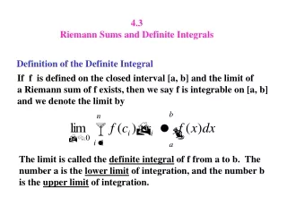
Definite Integrals To define the definite integral, consider the following limit. To say that this limit exists means there exists a real number L such that for each ε> 0 there exists a > 0 so that for every partition with |||| < it follows that regardless of the choice of ci in the ith subinterval of each partition .
Definite Integrals Though Riemann sums were defined for functions with very few restrictions, a sufficient condition for a function f to be integrable on [a, b] is that it is continuous on [a,b].
Example 2 – Evaluating a Definite Integral as a Limit Evaluate the definite integral Solution: The function f(x) = 2x is integrable on the interval [–2, 1] because it is continuous on [–2, 1]. Moreover, the definition of integrability implies that any partition whose norm approaches 0 can be used to determine the limit.
Example 2 – Solution cont’d For computational convenience, define by subdividing [–2, 1] into n subintervals of equal width Choosing cias the right endpoint of each subinterval produces
Example 2 – Solution cont’d So, the definite integral is given by
Definite Integrals Because the definite integral in Example 2 is negative, it does not represent the area of the region shown in Figure 4.21. Definite integrals can be positive, negative, or zero. For a definite integral to be interpreted as an area, the function f must be continuous and nonnegative on [a, b], as stated in the following theorem. Figure 4.21
Definite Integrals Figure 4.22
Definite Integrals As an example of Theorem 4.5, consider the region bounded by the graph of f(x) = 4x – x2 and the x-axis, as shown in Figure 4.23. Because f is continuous and nonnegative on the closed interval [0, 4], the area of the region is Figure 4.23
Definite Integrals You can evaluate a definite integral in two ways—you can use the limit definition or you can check to see whether the definite integral represents the area of a common geometric region such as a rectangle, triangle, or semicircle.
Example 3 – Areas of Common Geometric Figures Sketch the region corresponding to each definite integral. Then evaluate each integral using a geometric formula. a. b. c.
Example 3(a) – Solution This region is a rectangle of height 4 and width 2. Figure 4.24(a)
Example 3(b) – Solution cont’d This region is a trapezoid with an altitude of 3 and parallel bases of lengths 2 and 5. The formula for the area of a trapezoid is h(b1 + b2). Figure 4.24(b)
Example 3(c) – Solution cont’d This region is a semicircle of radius 2. The formula for the area of a semicircle is Figure 4.24(c)
Properties of Definite Integrals The definition of the definite integral of f on the interval [a, b] specifies that a < b. Now, however, it is convenient to extend the definition to cover cases in which a = b or a > b. Geometrically, the following two definitions seem reasonable. For instance, it makes sense to define the area of a region of zero width and finite height to be 0.
Example 4 – Evaluating Definite Integrals Evaluate each definite integral.
Example 4 – Solution a. Because the sine function is defined at x = π, and the upper and lower limits of integration are equal, you can write b. The integral is the same as that given in Example 2(b) except that the upper and lower limits are interchanged. Because the integral in Example 3(b) has a value of you can write
Example 4 – Solution cont’d In Figure 4.25, the larger region can be divided at x = c into two subregions whose intersection is a line segment. Because the line segment has zero area, it follows that the area of the larger region is equal to the sum of the areas of the two smaller regions. Figure 4.25
Properties of Definite Integrals Note that Property 2 of Theorem 4.7 can be extended to cover any finite number of functions.
Example 6 – Evaluation of a Definite Integral Evaluate using each of the following values. Solution:
Properties of Definite Integrals If f and g are continuous on the closed interval [a, b] and 0 ≤ f(x) ≤ g(x) for a≤ x ≤ b,the following properties are true. First, the area of the region bounded by the graph of f and the x-axis (between a and b) must be nonnegative.
Second, this area must be less than or equal to the area of the region bounded by the graph of g and the x-axis (between a and b ), as shown in Figure 4.26. These two properties are generalized in Theorem 4.8. Properties of Definite Integrals Figure 4.26