The Mundell-Fleming model

1. The Mundell-Fleming model From IS-LM to Mundell-Fleming Policy in an open economy

2. The Mundell-Fleming model • Last week we introduced the basic elements required to analyse an open economy • The current account: imports and exports • The capital account: saving/investment flows • The balance of payments equilibrium as a combination of the two • The role of exchange rates

3. The Mundell-Fleming model • This week we integrate these elements into the Mundell-Fleming model, which is an IS-LM model extended to account for imports and exports • Although this will not be covered, in theory this can be used in turn to modify the AS-AD model to account for international trade with inflation • As we saw last week, the price level can be included through the analysis of real exchange rates

4. The Mundell-Fleming model From IS-LM to the Mundell-Fleming model Effectiveness of policy

5. From IS-LM to Mundell-Fleming • Model developed by Robert Mundell and Marcus Fleming • It extends the IS-LM model to an open economy • Aggregate demand now contains the current account : i.e. the difference between exports and imports. • X(Y*,e) : Exports are a function of the income of the rest of the world (exogenous) and the exchange rate • M(Y,e) : Importations are a function of national income and the exchange rate

6. From IS-LM to Mundell-Fleming Determinants of the current account: • If e falls (depreciation): exportations are more competitive and imports more expensive. The net balance of the current account increases. • If Y increases: imports increase and the net balance of the current account falls. • Y* is exogenous, and Y is already determined in IS-LM. There is an extra variable to account for: the exchange rate e. • We need to add another equation (market) in order to be able to solve the system: we use the equilibrium condition on the balance of payments

7. From IS-LM to Mundell-Fleming • Reminder: the balance of payments is the sum of the current account and the capital account: • The equilibrium exchange rate is achieved when BP is equal to zero, in other words when the deficits and surpluses of the two accounts compensate exactly. • One can see that this equilibrium condition can be expressed in the (Y,i) space of IS-LM. • We still need to relate the exchange rate e to these variables

8. From IS-LM to Mundell-Fleming • The capital account (KA) • Is in surplus if the inflows of capital are larger than the outflows. • Is in deficit in the other case. • What determines these capital flows ? • Intuitive answer: the earnings on savings • If savings earn a higher return in Europe compared to the USA, one would expect American capital to flow towards Europe.

9. From IS-LM to Mundell-Fleming • Investors choose between assets that pay different interest rates in different currencies. • What is the expected return for each of the possible investment? • Their decision needs to account for the interest rate differentials… • …But also for the evolution of the exchange rates between currencies. • This arbitrage mechanism produces what is called the uncovered interest rate parity (UIRP) • This gives us a relation between interest rate differentials and changes in the exchange rate

10. From IS-LM to Mundell-Fleming • You are a European investor with capital K (in €) looking for a 1-year investment. • You can invest in €-denominated bonds, and after a year you earn: • Or you can buy $-denominated US bonds: • Step 1: you first convert your capital into dollars: • Step 2: after a year, you’ve earned (in dollars):

11. From IS-LM to Mundell-Fleming • But you need to bring you investment back home ! • In other words you need to convert your capital in $ back into €. • In the mean time the $/€ exchange rate may have changed • Step 3: you convert your investment into € • You are indifferent if the 2 returns are equal

12. From IS-LM to Mundell-Fleming • You’re indifferent between $ and € assets if: • Rearranging gives: • If the exchange rate is not too volatile, this can be expressed as:

13. Expected exchange rate depreciation Home interest rate World interest rate From IS-LM to Mundell-Fleming • Let’s summarise: Capital flows ensure an equalisation of interest rates expressed in the same currency • If the home interest rate is higher than world interest rate, zero net capital flows between countries requires investors to be expecting a depreciation of the home currency. • If this is not the case, then capital will flow into the home country, appreciating e until depreciation expectations occur • Only if the home rate equals the foreign rate will depreciation/appreciation expectations be zero (equilibrium)

14. From IS-LM to Mundell-Fleming • On BP the balance of payments is in equilibrium i BoP surplus Appreciation of e • BP is upward-sloping • An increase in Y leads to a BoP deficit (CA deficit) • Returning to equilibrium requires a KA surplus, and hence a higher i BP KA surplus • The slope depends on the international mobility of capital • The lower capital mobility, the larger the slope of BP. CA deficit BoP deficit Depreciation of e Y

15. BP From IS-LM to Mundell-Fleming • The MF model was developed in the 60’s, when capital mobility was low (Bretton Woods) Perfect capital mobility i=i* i BoP Surplus Appreciation of e • As a simplification, nowadays we assume perfect capital mobility i* • However, this remains a simplification! • For certain cases (like the case of trade with China), The concept of imperfect capital mobility remains relevant. BoP Deficit Depreciation of e Y

16. From IS-LM to Mundell-Fleming • We now have 3 curves, IS-LM-BP : i LM BP i* IS Y

17. The Mundell-Fleming model From IS-LM to the Mundell-Fleming model Effectiveness of policy

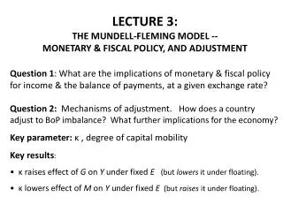
18. The effectiveness of policy • We now move to assessing the effectiveness of policy under the possible exchange rate settings:

19. The effectiveness of policy • Monetary policy with fixed exchange rate: i • LM shifts to the right • The increase in the money supply lowers the rate of interest, leading to depreciation pressures on e LM BP • In order to guarantee the fixed exchange rate the CB must immediately increase i to i=i* by reducing money supply i* IS • Such a policy cannot be carried out in practice Y

20. The effectiveness of policy • Fiscal policy with fixed exchange rate: i • IS shifts to the right: • The crowding out effect increases the rate of interest, creating appreciation pressures on e LM BP • In order to guarantee the fixed exchange rate the CB must immediately reduce i to i=i* by increasing money supply i* IS • Policy is effective in increasing Y Y

21. The effectiveness of policy • Monetary policy with flexible exchange rate: i • LM shifts to the right • The interest rate falls, which leads to a depreciation of the exchange rate e LM • The depreciation of the exchange rate stimulates exports and penalises imports • As a resut IS shifts to the right BP i* IS • Policy is effective Y

22. The effectiveness of policy • Fiscal policy with flexible exchange rate: i • IS shifts to the right • The Central Bank doesn’t have to react: The interest rate increases and the exchange rate appreciates LM BP • The appreciation of the exchange rate penalises exports and stimulates imports • IS shifts left i* IS • Policy is ineffective Y

23. The effectiveness of policy • Summarising all this: • Even with this simple example (assumption of perfect capital mobility), one can see that the effectiveness of policy depends on international conditions!

24. The effectiveness of policy Monetary Union Incompatibility Triangle (Mundell) Capital mobility Fixed exchange rate Flexible Exchange rate Financial Autarky Autonomous monetary policy