Download
1 / 22
220 likes | 331 Views
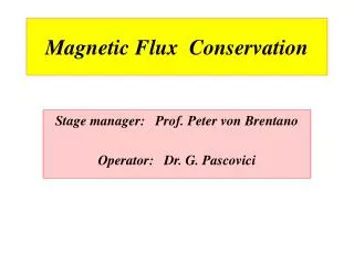
Magnetic Flux Conservation. Stage manager: Prof. Peter von Brentano Operator: Dr. G. Pascovici. What is electromagnetism?. The study of Maxwell’s equations, devised in 1863

E N D
Magnetic Flux Conservation Stage manager: Prof. Peter von Brentano Operator: Dr. G. Pascovici
What is electromagnetism? • The study of Maxwell’s equations, devised in 1863 to represent the relationships between electric and magnetic fields in the presence of electric charges and currents, whether steady or rapidly fluctuating, in a vacuum or in matter. • The equations represent one of the most elegant and concise way to describe the fundamentals of electricity and magnetism. They pull together in a consistent way earlier results known from the work of Gauss, Faraday, Ampère, Biot, Savart and others. • Remarkably, Maxwell’s equations are perfectly consistent with the transformations of special relativity.
Maxwell’s Equations E = electric field D = electric displacement H = magnetic field B = magnetic flux density = charge density j = current density 0 (permeability of free space) = 4 10-7 0 (permittivity of free space) = 8.854 10-12 c (speed of light) = 2.99792458 108 m/s
Maxwell 1: Equivalent to Gauss’ Flux Theorem: The flux of electric field out of a closed region is proportional to the total electric charge enclosed within the surface. A point charge q generates an electric field Area integral gives a measure of the net charge enclosed; divergence of the electric field gives the density of the sources.
Johann Carl Friedrich Gauss(30 April 1777 – 23 February 1855)
Maxwell 2: Gauss’ law for magnetism: The net magnetic flux out of any closed surface is zero. Surround a magnetic dipole with a closed surface. The magnetic flux directed inward towards the south pole will equal the flux outward from the north pole. If there were a magnetic monopole source, this would give a non-zero integral. Gauss’ law for magnetism is then a statement that: There are no magnetic monopoles
Maxwell 3: Equivalent to Faraday’s Law of Induction: (for a fixed circuit C) The electromotive force round a circuit =E.dl is proportional to the rate of change of flux of magnetic field =B.dS through the circuit. Faraday’s Law is the basis for electric generators. It also forms the basis for inductors and transformers. N S
Magnetic Flux • Magnetic Flux Illustrations • The contribution to magnetic flux for a given area is equal to the area times the component of magnetic field perpendicular to the area. • For a closed surface, the sum of magnetic flux is always equal to zero ( Gauss’ law for magnetism). • No matter how small the volume, the magnetic sources are always dipole sources (like miniature bar magnets), so that there are as many magnetic field lines coming in (to the south pole)
Maxwell 4: Originates from Ampère’s (Circuital) Law : Satisfied by the field for a steady line current (Biot-Savart Law, 1820):
A set of coils from 3xA to 0.25xA N.B. due to a very accurate technology the reproducibility of the number complete turns is ~ 10 -4
View of the experimental set-up with one large coil for all ferrite cores (from 3xA to 0.25xA 3xA 2xA 1xA 0.3xA Disadvantage: nonlinearity due to the influence of “escape magnetic lines” for the smaller cores < 3A
Individual coils for each of the ferrite cores (from 3xA to 0.25xA) Advantage: smaller errors due to the very small influence of “escape magnetic lines” ( mainly for the smaller cores << 3 A)
Two experimental methods (set-up) a) Individual coils for each core (from 0.25A to 3A) - sinusoidal generator ( 40 Hz-5 kHz ) - amplitudes . 0.5 to 3 V rms. - accurate sinusoidal U1/U2 oscillations ( the sum of all harmonics < 5%) - frequency range 50 to 500 Hz Experimental results: - the mean variation of the U1/U2 ration is less then 3.5 x 10(-4) from 0.45A up to 3A
One single large coil (3A) for all cores from 0.25 to 3A - sinusoidal generator ( 40 Hz-5 kHz ) - amplitudes . 0.5 to 3 V rms. - accurate sinusoidal U1/U2 oscillations ( the sum of all harmonics < 5%) - frequency range 50 to 500 Hz Experimental results: - the mean variation of the U1/U2 ration is less then 2.5 x 10(-3) from 0.45A up to 3A N.B. the very small core 0.25A showed a larger deviation, namely ~ 7 x 10(-3)
Individual coils for each of the ferrite cores (from 3xA to 0.3xA) Advantage: smaller errors due to the very small influence of “escape magnetic lines” ( mainly for the smaller cores << 3 A)
View of experimental set-up with individual coils for each ferrite core (from 3xA to 0.3xA)