Download
1 / 56
570 likes | 728 Views
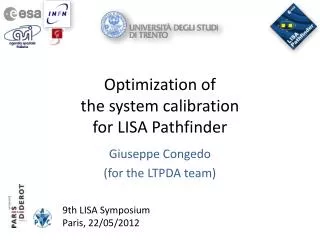
PhD oral defense 26th March 2012. Spacetime metrology with LISA Pathfinder. Giuseppe Congedo. LISA Pathfinder. Test Mass. vibration tests. Optical Bench. Partenership of many universities world wide Univ. of Trento plays the role of Principal Investigator

E N D
PhD oral defense 26th March 2012 Spacetime metrology with LISA Pathfinder Giuseppe Congedo
LISA Pathfinder Test Mass vibration tests Optical Bench • Partenership of many universities world wide • Univ. of Trento plays the role of Principal Investigator • Currently in the final integration • Planned to flight in the next years Housing courtesy of SpaceCraft Giuseppe Congedo - PhD oral defense
Outline of the talk In the framework of this ESA mission, we talk about: • Theoretical characterization of the LISA arm without/with noise • Dynamical modeling for LISA Pathfinder, closed-loop equations of motion • Data analysis: simulation and analysis of some experiments, system calibration, estimation of the acceleration noise, ... Giuseppe Congedo - PhD oral defense
LISA, a space-borne GW detector LISA measures the relative velocities between the Test Masses (TMs) as Doppler frequency shifts LISA is the proposed ESA-NASA mission for GW astrophysics in 0.1 mHz – 0.1 Hz • astrophysical sources at cosmological distances • merger of SMBHs in galactic nuclei • galactic binaries (spatially resolved and unresolved) • EMRIs • GW cosmic background radiation SpaceCraft (SC) Test Mass Optical Bench Giuseppe Congedo - PhD oral defense
LISA Pathfinder,in-flight test of geodesic motion • Down-scaled version of LISA arm~40 cm • In-flight test of the LISA hardware (sensors, actuators and controllers) • Prove geodesic motion of TMs to within 3x10-14 ms-2/√Hz @1mHzdifferential acceleration noise requirement • Optically track the relative motion to within 9x10-12 m/√Hz @1mHz differential displacement noise ~40 cm ~5 cm Giuseppe Congedo - PhD oral defense
LISA Pathfinder,in-flight test of geodesic motion Residual acceleration noise 9x10-12 m/√Hz ~ 1 order of magnitude relaxation 3x10-14 ms-2/√Hz Giuseppe Congedo - PhD oral defense
Spacetime metrology without noise How does the LISA arm work? It is well-known in General Relativity that the Doppler frequency shift measured between an emitter sending photons to a receiver – we name it Doppler link – is The differential operator implementing the parallel transport of the emitter 4-velocity along the photon geodesic can be defined as and one can show that it is given by • The Doppler link measures • relative velocity between the particles (without parallel transport) • the integral of the affine connection (i.e., curvature + gauge effects) Giuseppe Congedo - PhD oral defense
Doppler link as differential accelerometer The Doppler link (and the LISA arm) can be reformulated as a differential time-delayed accelerometer measuring: • The spacetime curvature along the beam • Parasitic differential accelerations • Gauge “non-inertial” effects For low velocities and along the optical axis, differentiating the Doppler link it turns out ~ω/c (1,1,0,0) d\dτ ~(c,0,0,0) to 1st order Giuseppe Congedo - PhD oral defense
Doppler response to GWs in the weak field limit To prove that this reasoning is correct, it is possible to evaluate the Doppler response to GWs in the TT gauge obtaining the standard result already found in literature where h is the “convolution” with the directional sensitivities and the GW polarizations The parallel tranport induces a time delay to the time of the emitter Giuseppe Congedo - PhD oral defense
Noise sources within the LISA arm • LPF is a down-scaled version of the LISA arm, which is a sequence of 3 measurements: • In LISA there are 3 main noise sources: • laser frequency noise from armlength imbalances, compensated by TDI, not present in LPF • parasitic differential accelerations, characterized with LPF • sensing noise (photodiode readout), characterized with LPF Giuseppe Congedo - PhD oral defense
Laser frequency noise In space, laser frequency noise can not be suppressed as on-ground: arm length imbalances of a few percent produce an unsuppressed frequency noise of 10-13/√Hz (2x10⁻⁷ ms-2/√Hz) @1mHz σ1 Doppler links Time-Delay Interferometry (TDI) suppresses the frequency noise to within 10-20/√Hz (2x10-15 ms-2/√Hz) @1mHz It is based upon linear combinations of properly time delayed Doppler links X1 σ1' Giuseppe Congedo - PhD oral defense
Total equivalent acceleration noise • Differential forces (per unit mass) between the TMs, due to electromagnetics & self-gravity within the SC, • Sensing noise (readout, optical bench misalignments), We can express all terms as total equivalent acceleration noise will be demonstrated by LPF to be within 3x10-14 ms-2/√Hz@1mHz total equivalent acceleration noise sensing forces Giuseppe Congedo - PhD oral defense
Dynamics of fiducial points • Fiducial points are the locations on TM surface where light reflects on • They do not coincide with the centers of mass • As the TMs are not pointlike, extended body dynamics couples with the differential measurement (cross-talk) Local link Link between the SCs Giuseppe Congedo - PhD oral defense
LISA Technology Package We switch to the real instrument... 15 control laws are set up to minimize: SC jitter and differential force disturbances Giuseppe Congedo - PhD oral defense
Degrees of freedom • Science mode, along the optical axis x: • TM1 is in free fall • the SC is forced to follow TM1 through thruster actuation • TM2 is forced to follow TM1 through capacitive actuation Giuseppe Congedo - PhD oral defense
Closed-loop dynamics • In LPF dynamics: • the relative motion is expected to be within ~nm • we neglect non-linear terms from optics and extended body Euler dynamics • the forces can be expanded to linear terms Since the linearity of the system, it follows that the equations of motion are linear, hence in frequency domain they can be expressed in matrix form (for many dofs) Dynamics operator Giuseppe Congedo - PhD oral defense
Closed-loop dynamics As said, the equations of motion are linear and can be expressed in matrix form Dynamics “forces produce the motion” Sensing “positions are sensed” Control “noise, actuation and control forces” The generalized equation of motion in the sensed coordinates where the 2nd-order differential operator is defined by Giuseppe Congedo - PhD oral defense
Dynamical model along the optical axis direct forces on TMs and SC • force gradients guidance signals: reference signals that the controllers must follow (“the loops react”) • sensing cross-talk • actuation gains Giuseppe Congedo - PhD oral defense
Dynamical model along the optical axis The model along x can be mapped to the matrix formalism... Giuseppe Congedo - PhD oral defense
Two operators The differential operator • estimates the out-of-loop equivalent acceleration from the sensed motion • subtracts known force couplings, control forces and cross-talk • subtracts system transients The transfer operator • solves the equation of motion for applied control bias signals • is employed for system calibration, i.e. system identification Giuseppe Congedo - PhD oral defense
Suppressing system transients The dynamics of LPF (in the sensed coordinates) is described by the following linear differential equation • Particular solution (steady state): • depends on the applied forces • can be solved in frequency domain • Homogeneous solution (transient state): • depends on non-zero initial conditions • is a combination of basis functions Giuseppe Congedo - PhD oral defense
Suppressing system transients Applying the operator on the sensed coordinates, transients are suppressed in the estimated equivalent acceleration But, imperfections in the knowledge of the operator (imperfections in the system parameters) produce systematic errors in the recovered equivalent acceleration System identification helps in mitigating the effect of transients Giuseppe Congedo - PhD oral defense
Cross-talk from other degrees of freedom Beyond the dynamics along the optical axis... cross-talk from other DOFs nominal dynamics along x All operators can be expanded to first order as “imperfections” to the nominal dynamics along x To first order, we consider only the cross-talk from a DOF to x, and not between other DOFs. Cross-talk equation of motion Giuseppe Congedo - PhD oral defense
Data analysis during the mission • The Science and Technology Operations Centre (STOC): • interface between the LTP team, science community and Mission Operations • telecommands for strong scientific interface with the SpaceCraft • quick-look data analysis Giuseppe Congedo - PhD oral defense
Data analysis during the mission Data for this thesis were simulated with both analytical simplified models and the Off-line Simulation Environment – a simulator provided by ASTRIUM for ESA. It is realistic as it implements the same controllers, actuation algorithms and models a 3D dynamics with the couplings between all degrees of freedom • During operational exercises, the simulator is employed to: • check the mission timeline and the experiments • validate the noise budget and models • check the procedures: system identification, estimation of equivalent acceleration, etc. • Data were analyzed with the LTP Data Analysis Toolbox – an object-oriented Matlab environment for accountable and reproducible data analysis. initial splash screen Giuseppe Congedo - PhD oral defense
Multi-input/Multi-Output analysis We are able to recover the information on the system by stimulating it along different inputs oi,1 oi,12 o1 fi,1 LPF dynamical system o12 fi,12 fi,SC ... In this work two experiments were considered allowing for the determination of the system: ... Exp. 1: injection into drag-free loop Exp. 2: injection into elect. suspension loop Giuseppe Congedo - PhD oral defense
LPF model along the optical axis • For simulation and analysis, we employ a model along the optical axis • Transfer matrix (amplitude/phase) modeling the system response to • applied control guidance signals “the spacecraft moves”: drag-free loop “the second test mass moves”: suspension loop cross-talk Giuseppe Congedo - PhD oral defense
LPF parameters along the optical axis Giuseppe Congedo - PhD oral defense
Equivalent acceleration noise Current best estimates of the direct forces from on-ground measurements Relative acceleration between the TMs • at high frequency, dominated by sensing • at low frequency, dominated by direct forces Goal: prove the relevance of system identification for the correct assessement of the equivalent acceleration noise Giuseppe Congedo - PhD oral defense
Estimation of equivalent acceleration noise system identification optimal design with system identification parameters ω12, ω122, S21, Adf, ... equivalent acceleration sensed relative motion o1, o12 diff. operator Δ without system identification Giuseppe Congedo - PhD oral defense
Identification experiment #1 Exp. 1: injection of sine waves into oi,1 • injection into oi,1 produces thruster actuation • o12 shows dynamical cross-talk of a few 10-8 m • allows for the identification of: Adf, ω12, Δt1 Giuseppe Congedo - PhD oral defense
Identification experiment #2 Exp. 2: injection of sine waves into oi,12 • injection into oi,1 produces capacitive actuation on TM2 • o1 shows negligible signal • allows for the identification of: Asus, ω122, Δt2, S21 Giuseppe Congedo - PhD oral defense
Parameter estimation • Non-linear optimization: • preconditioned conjugate gradient search explores the parameter space to large scales • derivative-free simplex improves the numerical accuracy locally • Method extensively validated through Monte Carlo simulations cross-PSD matrix residuals Joint (multi-experiment/multi-outputs) log-likelihood for the problem Giuseppe Congedo - PhD oral defense
Non-Gaussianities Investigated the case of non-gaussianities (glitches) in the readout producing fat tails in the statistics (strong excess kurtosis) Better weighting for large deviations than squared and abs dev. Regularize the log-likelihood with a weighting function mean squared dev. (aka, “ordinary least squares”), Gaussian distr. abs. deviation, log-normal distr. log. deviation, Lorentzian distr. Giuseppe Congedo - PhD oral defense
Non-Gaussianities o12 • χ2 regularizes toward ~1 • the parameter bias, in average, tends to <3 Giuseppe Congedo - PhD oral defense
Under-performing actuators under-estimated couplings Investigated the case of a miscalibrated LPF mission, in which: • the TM couplings are stronger than one may expect • the (thruster and capacitive) actuators have an appreciable loss of efficiency The parameter bias reduces from 103-104σ to <2 and the χ2 from ~105 to ~1 Giuseppe Congedo - PhD oral defense
Under-performing actuators under-estimated couplings Exp. 1 residuals ~2 orders of magnitude ~3 orders of magnitude Exp. 2 residuals Giuseppe Congedo - PhD oral defense
Equivalent acceleration noise Inaccuracies in the estimated system parameters produce systematic errors in recovered equivalent acceleration noise PSD matrix of the sensed relative motion inaccuracies of the diff. operator “true” diff. operator, as with the perfect knowledge of the system systematic errors in the estimated equivalent acceleration noise • Perform an estimation of the equivalent acceleration noise in a miscalibrated LPF mission (as in the previous example): • without a system identification (@ initial guess) • with a system identification (@ best-fit) • with the perfect knowledge of the system (@ true) Giuseppe Congedo - PhD oral defense
Equivalent acceleration noise Blue: estimated without sys. ident. Dashed red: estimated with sys. ident. Black: “true” shape Estimated differential acceleration noise Δa~1.5x10⁻¹³ m s-2 Hz-1/2 • Thanks to system identification: • the estimated acceleration recovers the “true” shape • improvement of a factor ~2 around 50 mHz • improvement of a factor ~4 around 0.4 mHz Giuseppe Congedo - PhD oral defense
Equivalent acceleration noise Dashed green: estimated model without sys. ident. Solid green: estimated model with sys. ident. Solid black: “true” model Estimated differential acceleration noise and models Δa~1.5x10⁻¹³ m s-2 Hz-1/2 • The agreement between estimated noise and models shows: • the models explain the estimated acceleration spectra • the accuracy of the noise generation Giuseppe Congedo - PhD oral defense
Equivalent acceleration noise Solid red: TM-SC coupling forces Dashed red: capacitive actuation noise Solid black: thruster actuation noise Dashed black: o12 sensing noise Estimated differential acceleration noise and models plus fundamental sources Δa~1.5x10⁻¹³ m s-2 Hz-1/2 • The systematic errors are due to: • 0.4 mHz, uncalibrated coupling forces (ω12 and ω22) and capacitive actuation (Asus) • 50 mHz, uncalibrated thruster actuation (Adf) and sensing noise (S21) Giuseppe Congedo - PhD oral defense
Suppressing transients in the acceleration noise As a consequence of changes of state and non-zero initial conditions, the presence of transients in the data is an expected behavior. Transients last for about 2 hours in o12 Giuseppe Congedo - PhD oral defense
Suppressing transients in the acceleration noise Comparison: (i) between the acceleration estimated at the transitory (first 3x10⁴ s) and steady state; (ii) between the acceleration estimated without and with system identification Dashed: steady state Solid: transitory Blue: without sys. ident. Red: with sys. ident. Data simulated with ESA simulator: suppression is not perfect since the limitation of the model System identification helps in mitigating the transitory in the estimated acceleration noise Giuseppe Congedo - PhD oral defense
Design of optimal experiments Goal: find optimal experiment designs allowing for an optimal determination of the system parameters • The LPF experiments can be optimized within the system contraints: • shape of the input signals • sensing range of the interferometer 100 µm • thruster authority 100 µN • capacitive authority 2.5 nN input signals: series of sine waves with discrete frequencies (we require integer number of cycles) • T < 3h (experiment duration): fixed • Ninj = 7: fixed to meet the exp. duration • δt = 1200 s (duration of each sine wave): fixed • δtgap = 150 s (gap between two sine waves): fixed for transitory decay • fn (injection freq.): optimized • an (injection ampl.): varied according to fn and the (sensing/actuation) contraints Giuseppe Congedo - PhD oral defense
Design of optimal experiments Fisher information matrix noise cross PSD matrix input parameters (injection frequencies) estimated system parameters input signals being optimized modeled transfer matrix with system identification Perform (non-linear discrete) optimization of the scalar estimator optimization criteria minimizes “covariance volume” Giuseppe Congedo - PhD oral defense
Design of optimal experiments • With the optimized design: • Improvement in precision: • factor 2 for ω12 and ω122 • factor 4 for S21 • factor 5-7 for Asus, Adf : important for compensating the SC jitter • Some parameters show lower correlation than the standard experiments • The optimization converged to only two injection frequencies (0.83 mHz, 50 mHz) Giuseppe Congedo - PhD oral defense
Concluding remarks • Theoretical contribution to the foundations of spacetime metrology with the LPF differential accelerometer • Modeling of the dynamics of the LISA arm implemented in LPF • Development of the parameter estimation method employed for system calibration and subtraction of different effects • Relevance of system identification for LPF Giuseppe Congedo - PhD oral defense
Future perspectives • More investigation in the reformulation of the Doppler link as a differential accelerometer • Application of system identification to the analysis of some cross-talk experiments • Investigation of non-stationary (transient) components in the noise • Application of the proposed optimal design to the ESA simulator • Currently under investigation, the application of system identification in the domain of equivalent acceleration Giuseppe Congedo - PhD oral defense
Thanks for your attention! Giuseppe Congedo - PhD oral defense
Additional slides... Giuseppe Congedo - PhD oral defense