Download
1 / 43
430 likes | 529 Views
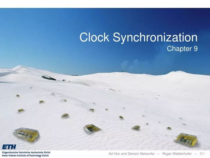
Clock Synchronization Chapter 9. TexPoint fonts used in EMF. Read the TexPoint manual before you delete this box.: A A A A A. Clock Synchronization. Rating. Area maturity Practical importance Theory appeal.

E N D
Clock SynchronizationChapter 9 TexPoint fonts used in EMF. Read the TexPoint manual before you delete this box.: AAAAA
Rating • Area maturity • Practical importance • Theory appeal First steps Text book No apps Mission critical Boooooooring Exciting
Overview • Motivation • Clock Sources & Hardware • Single-Hop Clock Synchronization • Clock Synchronization in Networks • Protocols: RBS, TPSN, FTSP, GTSP • Theory of Clock Synchronization • Protocol: PulseSync
Motivation • Synchronizing time is essential for many applications • Coordination of wake-up and sleeping times (energy efficiency) • TDMA schedules • Ordering of collected sensor data/events • Co-operation of multiple sensor nodes • Estimation of position information (e.g. shooter detection) • Goals of clock synchronization • Compensate offset* between clocks • Compensate drift* between clocks • *terms are explained on following slides Localization Sensing Duty-Cycling TDMA Time Synchronization
Properties of Clock Synchronization Algorithms • External versus internal synchronization • External sync: Nodes synchronize with an external clock source (UTC) • Internal sync: Nodes synchronize to a common time • to a leader, to an averaged time, or to anything else • One-shot versus continuous synchronization • Periodic synchronization required to compensate clock drift • A-priori versus a-posteriori • A-posteriori clock synchronization triggered by an event • Global versus local synchronization (explained later) • Accuracy versus convergence time, Byzantine nodes, …
Clock Sources • Radio Clock Signal: • Clock signal from a reference source (atomic clock) is transmitted over a long wave radio signal • DCF77 station near Frankfurt, Germany transmits at 77.5 kHz with a transmission range of up to 2000 km • Accuracy limited by the distance to the sender, Frankfurt-Zurich is about 1ms. • Special antenna/receiver hardware required • Global Positioning System (GPS): • Satellites continuously transmit own position and time code • Line of sight between satellite and receiver required • Special antenna/receiver hardware required
Clock Sources (2) • AC power lines: • Use the magnetic field radiating from electric AC power lines • AC power line oscillations are extremely stable (10-8 ppm) • Power efficient, consumes only 58 μW • Single communication round required to correctphase offset after initialization • Sunlight: • Using a light sensor to measure the length of a day • Offline algorithm for reconstructing global timestamps by correlating annual solar patterns (no communication required)
Clock Devices in Sensor Nodes • Structure • External oscillator with a nominal frequency (e.g. 32 kHz or 7.37 MHz) • Counter register which is incremented with oscillator pulses • Works also when CPU is in sleep state 7.37 MHz quartz 32 kHz quartz Mica2 TinyNode 32 kHz quartz
Clock Drift • Accuracy • Clock drift: random deviation from the nominal rate dependent on power supply, temperature, etc. • E.g. TinyNodes have a maximum drift of 30-50 ppm at room temperature rate This is a drift of up to 50 μs per second or 0.18s per hour 1+² 1 1-² t
Time accor- t t B ding to B 2 3 Answer Request from A from B t Time accor- t A ding to A 1 4 Sender/Receiver Synchronization • Round-Trip Time (RTT) based synchronization • Receiver synchronizes to the sender‘s clock • Propagation delay and clock offset can be calculated
Messages Experience Jitter in the Delay • Problem: Jitter in the message delay • Various sources of errors (deterministic and non-deterministic) • Solution: Timestamping packets at the MAC layer (Maróti et al.) • → Jitter in themessagedelayisreducedto a fewclockticks 1-10 ms 0-100 ms 0-500 ms Send Access Transmission timestamp Reception Receive 0-100 ms t timestamp
Some Details • Different radio chips use different paradigms: • Left is a CC1000 radio chip which generates an interrupt with each byte. • Right is a CC2420 radio chip that generates a single interrupt for the packet after the start frame delimiter is received. • In sensor networks propagationcan be ignored (<1¹s for 300m). • Still there is quite some variancein transmission delay because oflatencies in interrupt handling (picture right).
Symmetric Errors • Many protocols don’t even handle single-hop clock synchronization well. On the left figures we see the absolute synchronization errors of TPSN and RBS, respectively. The figure on the right presents a single-hop synchronization protocol minimizing systematic errors. • Even perfectly symmetric errors will sum up over multiple hops. • In a chain of n nodes with a standard deviation ¾ on each hop, the expected error between head and tail of the chain is in the order of ¾√n.
= + + + + t t S A P R 2 1 S S S , A A = + + + + t t S A P R 3 1 S S S , B B q = - = - + - t t ( P P ) ( R R ) 2 3 S , A S , B A B Reference-Broadcast Synchronization (RBS) • A sender synchronizes a set of receivers with one another • Point of reference: beacon’s arrival time A S B • Only sensitive to the difference in propagation and reception time • Time stamping at the interrupt time when a beacon is received • After a beacon is sent, all receivers exchange their reception times to calculate their clock offset • Post-synchronization possible • E.g., least-square linear regression to tackle clock drifts • Multi-hop?
0 1 1 1 2 2 2 2 Time-sync Protocol for Sensor Networks (TPSN) • Traditional sender-receiver synchronization (RTT-based) • Initialization phase: Breadth-first-search flooding • Root node at level 0 sends out a level discovery packet • Receiving nodes which have not yet an assigned level set their levelto +1 and start a random timer • After the timer is expired, a new level discovery packet will be sent • When a new node is deployed, it sends out a level request packet after a random timeout • Why this random timer?
Time-sync Protocol for Sensor Networks (TPSN) • Synchronization phase • Root node issues a time sync packet which triggers a random timer at all level 1 nodes • After the timer is expired, the node asks its parent for synchronization using a synchronization pulse • The parent node answers with an acknowledgement • Thus, the requesting node knows the round trip time and can calculate its clock offset • Child nodes receiving a synchronization pulse also start a random timer themselves to trigger their own synchronization 0 Time Sync 1 B ACK Sync pulse 1 2 A 2 2
= + + + + t t S A P R 0 2 1 A A A , B B = + + + + t t S A P R 1 B 4 3 B B B , A A - + - + - + - ( S S ) ( A A ) ( P P ) ( R R ) 1 2 q = A B A B A , B B , A B A 2 A 2 2 Time-sync Protocol for Sensor Networks (TPSN) • Time stamping packets at the MAC layer • In contrast to RBS, the signal propagation time might be negligible • Authors claim that it is “about two times” better than RBS • Again, clock drifts are taken into account using periodical synchronization messages • Problem: What happens in a non-tree topology (e.g. grid)? • Two neighbors may have bad synchronization?
Flooding Time Synchronization Protocol (FTSP) • Each node maintains both a local and a global time • Global time is synchronized to the local time of a reference node • Node with the smallest id is elected as the reference node • Reference time is flooded through the network periodically • Timestamping at the MAC Layer is used to compensate for deterministic message delays • Compensation for clock drift between synchronization messages using a linear regression table reference node 0 4 5 1 7 6 3 2
Best tree for tree-based clock synchronization? • Finding a good tree for clock synchronization is a tough problem • Spanning tree with small (maximum or average) stretch. • Example: Grid network, with n = m2nodes. • No matter what tree you use, the maximumstretch of the spanning tree will always beat least m (just try on the grid figure right…) • In general, finding the minimum maxstretch spanning tree is a hard problem, however approximation algorithms exist [Emek, Peleg, 2004].
Variants of Clock Synchronization Algorithms Tree-like Algorithms Distributed Algorithms e.g. FTSP e.g. GTSP Bad local skew All nodes consistently average errors to all neigbhors
FTSP vs. GTSP: Global Skew • Network synchronization error (global skew) • Pair-wise synchronization error between any two nodes in the network FTSP (avg: 7.7 μs) GTSP (avg: 14.0 μs)
FTSP vs. GTSP: Local Skew • Neighbor Synchronization error (local skew) • Pair-wise synchronization error between neighboring nodes • Synchronization error between two direct neighbors: FTSP (avg: 15.0 μs) GTSP (avg: 2.8 μs)
Global vs. Local Time Synchronization • Common time is essential for many applications: • Assigning a timestamp to a globally sensed event (e.g. earthquake) • Precise event localization (e.g. shooter detection, multiplayer games) • TDMA-based MAC layer in wireless networks • Coordination of wake-up and sleeping times (energy efficiency) Global Local Local Local
Theory of Clock Synchronization • Given a communication network • Each node equipped with hardware clock with drift • Message delays with jitter • Goal: Synchronize Clocks (“Logical Clocks”) • Both global and local synchronization! worst-case (but constant)
Time Must Behave! • Time (logical clocks) should not be allowed to stand still or jump • Let’s be more careful (and ambitious): • Logical clocks should always move forward • Sometimes faster, sometimes slower is OK. • But there should be a minimum and a maximum speed. • As close to correct time as possible!
Formal Model • Hardware clock Hv(t) = s[0,t] hv(¿) d¿with clock rate hv(t)2 [1-²,1+²] • Logical clock Lv(∙) which increases at rate at least 1 and at most ¯ • Message delays 2 [0,1] • Employ a synchronization algorithm to update the logical clock according to hardware clock and messages from neighbors Clock drift ² is typically small, e.g. ² ¼10-4 for a cheap quartz oscillator Logical clocks with rate less than 1 behave differently (“synchronizer”) Neglect fixed share of delay, normalize jitter Hv Time is 152 Time is 140 Time is 150 Lv?
… Old clock value:x Clock value:D+x Old clock value:D+x-1 Old clock value:x+1 Synchronization Algorithms: An Example (“Amax”) • Question: How to update the logical clock based on the messages from the neighbors? • Idea: Minimizing the skew to the fastest neighbor • Set the clock to the maximum clock value received from any neighbor(if larger than local clock value) • forward new values immediately • Optimum global skew of about D • Poor local property • First all messages take 1 time unit… • …then we have a fast message! Allow¯ = 1 New time is D+x skew D! Fastest Hardware Clock New time is D+x Time is D+x Time is D+x Time is D+x
Synchronization Algorithms: Amax’ • The problem of Amax is that the clock is always increased to the maximum value • Idea: Allow a constant slack γ between the maximum neighbor clock value and the own clock value • The algorithm Amax’ sets the local clock value Li(t) to → Worst-case clock skew between two neighboring nodes is still Θ(D) independent of the choice of γ! • How can we do better? • Adjust logical clock speeds to catch up with fastest node (i.e. no jump)? • Idea: Take the clock of all neighbors into account by choosing the average value?
Local Skew: Overview of Results Everybody‘sexpectation, fiveyearsago („solved“) All natural algorithms [Locher et al., DISC 2006] Blocking algorithm Lower bound of logD/ loglogD[Fan & Lynch, PODC 2004] 1 logD √D D … Dynamic Networks![Kuhn et al., SPAA 2009] Kappa algorithm[Lenzen et al., FOCS 2008] Tight lower bound[Lenzen et al., PODC 2009]
Enforcing Clock Skew • Messages between two neighboring nodes may be fast in one direction and slow in the other, or vice versa. • A constant skew between neighbors may be „hidden“. • In a path, the global skew may be in the order of D/2. 2 3 4 5 6 7 u v 2 3 4 5 6 7 vs 2 3 4 5 6 7 2 3 4 5 6 7 2 3 4 5 6 7 2 3 4 5 6 7
Local Skew: Lower Bound (Single-Slide Proof!) Lv(t) = x + l0/2 hv = 1 Lv(t) = x hv = 1+² Higherclockrates l0 = D Lw(t) Lw(t) hw = 1 hw = 1 • Add l0/2 skew in l0/(2²) time, messing with clock rates and messages • Afterwards: Continue execution for l0/(4(¯-1)) time (all hx = 1) • Skew reduces by at most l0/4 at least l0/4 skew remains • Consider a subpath of length l1 = l0·²/(2(¯-1)) with at least l1/4 skew • Add l1/2 skew in l1/(2²)= l0/(4(¯-1)) time at least 3/4·l1 skew in subpath • Repeat this trick (+½,-¼,+½,-¼,…) log2(¯-1)/²D times Theorem: (log(¯-1)/²D) skew between neighbors
Surprisingly, up to small constants, the (log(¯-1)/²D)lower bound can be matched with clock rates 2 [1,¯] We get the following picture [Lenzen et al., PODC 2009]: In practice, we usually have 1/² ¼ 104 > D. In other words, our initial intuition of a constant local skew was not entirely wrong! Local Skew: Upper Bound ... because too large clock rates will amplify the clock drift ². We can have both smooth and accurate clocks!
Synchronizing Nodes • Sending periodic beacon messages to synchronize nodes Beacon interval B 100 130 reference clock 0 t t=100 t=130 t 1 J J jitter jitter
How accurately can we synchronize two Nodes? • Message delay jitter affects clock synchronization quality y 0 r ^ ^ ^ r r y(x) = r·x + ∆y relative clock rate(estimated) clock offset x ∆y J J 1 Beacon interval B
Clock Skew between two Nodes • Lower Bound on the clock skew between two neighbors • Error in the rate estimation: • Jitter in the message delay • Beacon interval • Number of beacons k • Synchronization error: y 0 r ^ ^ r r x ∆y J J 1 Beacon interval B
Multi-hop Clock Synchronization • Nodes forward their current estimate of the reference clock • Each synchronization beacon is affected by a random jitter J • Sum of the jitter grows with the square-root of the distance • stddev(J1 + J2 + J3 + J4 + J5 + ... Jd) = √d×stddev(J) ... 0 1 2 3 4 d J1 J2 J3 J4 J5 Jd Multi-hop: Single-hop:
Linear Regression (e.g. FTSP) • FTSP uses linear regression to compensate for clock drift • Jitter is amplified before it is sent to the next hop y 0 r Example for k=2 ^ synchronization error r ^ y(x) = r·x + ∆y clock offset relative clock rate(estimated) ∆y x J J 1 Beacon interval B
The PulseSync Protocol • Send fast synchronization pulses through the network • Speed-up the initialization phase • Faster adaptation to changes in temperature or network topology Beacon time B Beacon time B 0 0 1 1 FTSP 2 2 Expected time = D·B/2 3 3 4 4 t PulseSync Expected time = D·tpulse t tpulse
The PulseSync Protocol (2) • Remove self-amplification of synchronization error • Fast flooding cannot completely eliminate amplification y 0 r Example for k=2 synchronization error ^ r ^ y(x) = r·x + ∆y clock offset relative clock rate(estimated) ∆y x J J The green line is calculated using k measurement points that arestatistically independent of the red line. 1 Beacon interval B
FTSP vs. PulseSync • Global Clock Skew • Maximum synchronization error between any two nodes FTSP PulseSync
FTSP vs. PulseSync • Sychnronization Error vs. distance from root node FTSP PulseSync
Open Problem • As listed on slide 9/6, clock synchronization has lots of parameters. Some of them (like local/gradient) clock synchronization have only started to be understood. • Local clock synchronization in combination with other parameters are not understood well, e.g. • accuracy vs. convergence • fault-tolerance in case some clocks are misbehaving [Byzantine] • clock synchronization in dynamic networks