1 / 0

Unit 1 Introduction to DBMS

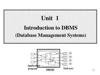
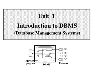
Unit 1 Introduction to DBMS. Common Terms. Data : collection of interrelated information about world being modeled DBMS : general-purpose software to define, create, modify, retrieve, delete and manipulate a database Goals: Efficient data management (faster than files) Large amount of data

seamus
Download Presentation

Unit 1 Introduction to DBMS

An Image/Link below is provided (as is) to download presentation Download Policy: Content on the Website is provided to you AS IS for your information and personal use and may not be sold / licensed / shared on other websites without getting consent from its author. Content is provided to you AS IS for your information and personal use only. Download presentation by click this link. While downloading, if for some reason you are not able to download a presentation, the publisher may have deleted the file from their server. During download, if you can't get a presentation, the file might be deleted by the publisher.

E N D

Presentation Transcript


  1. Unit 1Introduction to DBMS

  2. Common Terms Data: collection of interrelated information about world being modeled DBMS: general-purpose software to define, create, modify, retrieve, delete and manipulate a database Goals: Efficient data management (faster than files) Large amount of data High reliability Information sharing (multiple users)
  3. Data Abstraction Hiding system complexity and physical storage details from users and applications View 2 View n View1 Customized views Logical Level Conceptual representation Physical level Physical data description and storage
  4. Classification of DBMS Relational DBMS: Modeling concept: tables and constraints on tables Query Language: SQL Applications: suited for traditional business processing Object-Oriented DBMS Modeling concepts: objects, classes, inheritance Query Language: object oriented OQL Applications: suited for CAD databases, CASE databases Object-Relational DBMS: Incorporate OO concepts into relational model Similar functionality as OO-DBMS, but different implementations XML DBMS
  5. Entity-Relationship Model A schema in E/R
  6. E/R Model (Cont.) Entities: Represent objects Example: customers, accounts, bank branch Relationships: Associate entities Examples: Account “A-101” is held by customer “Johnson” Relationship set “depositor” associates customers with accounts Widely used for database design
  7. Relational Model Data represented as tables Attributes account- number street Customer-id city name Main Jamboree Culver Peltason Campus Johnson Smith Johnson Jones Smith A-101 A-215 A-201 A-217 A-201 Irvine Los Angeles San Diego Santa Ana Riverside 192-83-7465 019-28-3746 192-83-7465 321-12-3123 019-28-3746
  8. Sample Relational Database
  9. Schemas and Instances Schema: overall structure, and constraints over database changes infrequently Instance: data currently instantiated in database changes frequently Schema Instances Emp Tables Emp (ename, did) Dept(did, dname, mgr) Constraints each department has a single manager (John, 10), (Cindy, 15), (Martha, 10) Dept (10, Toy, John), (15, Sales, Cindy)
  10. DBMS Languages Data Definition Language (DDL) Used to describe a schema Data Manipulation Language (DML) Used by users to query the DB and change the data Storage Definition Language (SDL) Define the internal storage schema View Definition Language (VDL) Define views
  11. Data Definition Language (DDL) Specification notation for defining database schema CREATE TABLE account(accountID char(10), balance integer); DDL compiler generates metadata i.e., “data about data” Other info, such as indexes, constraints
  12. Data Manipulation Language (DML) Language for accessing and manipulating the data organized by the appropriate data model A query specifies what data is required Two classes of languages Procedural: user specifies how to get data Nonprocedural: user does not specify how to get data SQL is the most widely used query language
  13. SQL (Structured Query Language) Widely-used nonprocedural language “Find the name of the customer with id 192-83-7465.”SELECT customer-nameFROM customerWHERE customer-id = ‘192-83-7465’; Basic SQL has limited expressive power: Some functions cannot be implemented Application programs access DB through one of Language extensions to allow embedded SQL Application program interface (e.g. ODBC/JDBC) that allow SQL queries to be sent to a database
  14. DBMS Interface Provides users means to interact with database: Menu driven interface Graphical interface Forms based interface Natural Language Interface WWW connectivity.
  15. People Involved with DBMS DBMS designers and implementers Database administrator (DBA) “superuser” of a database, similar to a system administrator. Define schemas, views, authorization, indexes, tuning parameters, etc. Application programmers Online users Naïve users
  16. Database-design process Entity/Relationship Model Entity sets Relationship sets Constraints on entity sets Constraints on relationship sets Weak entity sets Superclass/subclass relationships Aggregation Good design Principles
  17. Database-Design Process Requirement Analysis Functional requirements Data requirements conceptual design logical design physical design functional analysis application design transaction implementation conceptual schema logical schema (in DBMS model) High-level specs application programs Physical schema Functional Design Database Design
  18. Database-Design Tools Help partially automate the design cycle. Graphical interface to specify conceptual schemas. Partially automated techniques to map to logical (DBMS dependent) model. Features of a good design tool: Iterative: errors/shortcomings of original design found later can be corrected without full restart. Interactive: any design choices made by system during design should be based on interaction with designer. Feedback: a designer’s change made at logical and/or physical levels should be automatically translated to changes at higher levels. Example design tools: Developer 2000 by Oracle, Rational Tools
  19. Entity/Relationship (E/R) Model Entities: objects Relationships: associate entities Roles of entities in a relationship Constraints on entities: domain constraints key constraints Constraints on relationships: Cardinality constraints Participation constraints Weak Entity Sets Multiway relationships Subclass/superclass Relationships Aggregation
  20. balance city street number name custacct id Entities and Entity Sets Entities: nouns, “things” in the world Have attributes: course name, id, address, dept, age, room, … Entity sets: a set of entities In OO terminology, entity set = “class,” and entity = “instance.” Customer Account
  21. Attributes Single-valued versus multi-valued: “telephone number”: multi-valued “Salary”: single-valued Atomic versus composite: “Age”: atomic “Address”: composite Derived versus stored: Derived: derived from other attributes or entities, e.g., “age” derived from “date of birth.” Stored: all other attributes
  22. Relationships Relationship: association of multiple entities Relationship Set: set of relationships over the same entity sets binary, ternary, 4-nary, …n-nary Custom-Account Relationship set account customer 259, 10K Tom, 62900, Main, LA 305, 20K Jane, 62901, North, Irvine 245, 2400 Visualizing relationships as a table. Each row: pair of entities participating in the relationship
  23. balance city street number name age Customer Account dob custacct id opendate tel ER Diagram Graphical representation of ER schema. Put as much information as possible. Entity set: rectangle Attribute: ellipse Derived attribute: dashed ellipse (“age”) Multivalued attribute: double ellipse (“tel”) Relationship set: diamond, with lines connected to its entity sets. May have attributes, called “relationship attributes.”
  24. balance number Key Constraints on Entity Sets Associate each entity set with a “key,” which is set of attributes that uniquely identify an entity in entity set. In ER diagram: denoted by underlining the attributes Multiple keys possible: One primary keyis chosen and underlined. Other keys, called secondary keys, either not indicated or listed in a side comment attached to the diagram. name dept course student Account No two students have the same name in the same dept. No two accounts have the same number.
  25. Domain Constraints on Entity Sets An attribute is associated with a domain. The value of the attribute for each entity is constrained to be in the domain only. Example: Gender: “F” or “M” Age: “> 20”
  26. A B B A B A Many-to-many Many-to-one One-to-one Cardinality Constraints Multiplicity of binary relationship set R between entity sets A and B Example: For “One-to-one,” an entity in A is associated with at most one entity in B, and vice versa. (A = B = “person”, R = “married-to”)
  27. Many-to-many Relationship custacct customer account legal opendate Multiple customers can share an account Many accounts may have one owner (We use customer names as the ids.) legal
  28. Many-to-One Relationship 1 N custacct customer account Illegal  opendate Multiple customers can share an account, but one customer can have only one account. Represented by an arrow pointing to “one.” Note: could have no account! legal
  29. Many-to-One Relationship (cont) custacct customer account opendate In a many-to-one relationship, relationship attributes can be repositioned to the entity set on the “many” side. custacct customer account opendate
  30. One-to-one Relationship custacct customer account opendate Illegal 1 customer can have (at most) 1 account. 1 account can be owned by (at most) 1 customer Relationship attributes “opendate” can be shifted to either entity set. One-to-one relationship is considered as a special case of many-to-one relationship Illegal Legal
  31. Participation Constraints Two kinds of participation constraints Total participation (also called existential dependency): each employee must belong to at least one department. Otherwise, partial participation. Belongs-to employee department
  32. Example amount loandid Ss# name borrower loan customer Belongs-to Customer-of branch Keys: ss#, loanid, branchid Cardinality constraint: each loan belongs to a single branch Participation constraints: --- Each customer must be a customer of at least one branch ---- Each loan must belong to at least one branch branchid location
  33. Weak Entity Sets Weak entity sets:they do not have sufficient attributes to form a key. They need to “borrow” attributes from other entity sets to form a key. Example: Transactions of different accounts could have the same trans#, so “trans#” cannot be a key By borrowing attribute “number” from “account,” we have a key for “transaction.” “Transaction” is a weak entity set related to accounts via log relationship. trans# number balance log transaction account
  34. Weak Entity Sets (cont’) A weak entity set depends upon (one or more) strong entity sets via a one-to-many relationship from whom they derive their key. The “helper” entity set that provides the attributes is called the “owner” entity set. A weak entity set may have a discriminator(or a partial key) that distinguish between weak entities related to the same strong entity Key of weak entity set = key of owner entity set(s) + discriminator trans# number balance amount log transaction account
  35. name SSN Multiway Relationships Usually binary relationships (connecting two E.S.) suffice. Sometimes we need more E.S. connected by one relationship. Similar to binary relationship, cardinality and participation constraints defined over multiway relationships CAB Relationship Set branch acct# CAB account customer balance
  36. name SSN Cardinality Constraints over Multiway Relationships Many-to-many-to-1 relationship Meaning: each (customer, account) determines the branch. Illegal: Jane has account 1001 at 2 branches branch acct# CAB account customer balance Legal
  37. name SSN Cardinality Constraints over Multiway Relationships Many-to-1-to-1 relationship Meaning: Each (customer, branch) related to a single account Each (customer, account) pair related to a single branch Illegal: Jane has 2 accounts in Tokyo Branch branch acct# CAB account customer balance Legal
  38. name SSN Cardinality Constraints over Multiway Relationships 1-to-1-to-1 relationship Meaning: Each (customer, branch) related to a single account Each (customer, account) pair related to a single branch Each (branch, account) pair can have single customer Illegal: Both Tom and Jane have account 1002 in Tokyo Branch branch acct# CAB account customer balance Legal
  39. (Strong) Entity Sets to Relations name ssno salary employee Relation: Employee(ssno, name, salary) Key: ssno
  40. Relationship Sets to Relations Relation: WorksOn(ssno,proj#,startdate) Key: ssno,proj# IND (INclusion Dependencies): workson[proj#] Í project[proj#] workson[ssno] Í employee[ssno] startdate name ssno salary Proj# mgr employee WorksOn project
  41. Multiway Relationships Relation: worksusing(ssno,proj#,toolid, startdate) Key: ssno,toolid IND: worksusing[proj#] Íproject[proj#] worksusing[ssno] Íemployee[ssno] worksusing[toolid] Ítools[toolid] employee[ssno] Í worksUsing[ssno] startdate name salary proj# mgr ssno WorksUsing project employee tool toolid spec
  42. Subclass/Superclass Relations: employee(ssno, name, salary) staff(ssno, position) faculty(ssno, rank) studentassistant(ssno, percentage_time) Key: ssno for all relations IND: staff[ssno] Íemployee[ssno] faculty[ssno] Íemployee[ssno] studentassistant[ssno] Íemployee[ssno] Cannot represent a total constraint. name salary ssno employee Isa faculty staff student assistant position Percentage Time rank
  43. Alternative design Relation: employee(ssno, name, salary, Isstaff, position, Isfaculty, rank, IsStudentassistant, percentage-time) Key : ssno IsStaff, IsFaculty, Isstudent_assistant are boolean values (either true or false). Contain many null values. Still cannot represent a total constraint. (We cannot say something like “One of IsStaff, IsFaculty, IsStudentassistant must be non NULL.”) name salary ssno employee Isa faculty staff Student assistant position Percentage Time rank
  44. Weak Entity Sets Relation: account(acct#,customer, balance) transaction(acct#,trans#, amount) Key of Transaction: acct#, trans# IND: transaction[acct#] Í account[acct#] No relation for the weak relationship set “Log.” Acct# trans# balance amount customer log transaction account
  45. Ternary  Binary Relationships branches branches CAB cannot be represented as the three binary relationships: Reason: the binary relationships cannot correctly capture the information represented by the ternary relationship. ?? CB AB CAB customers accounts CA customers accounts CB AB CA CAB relationships Relationships for the new ER diagram (after projections)
  46. Ternary  Binary Relationships branches branches But another set of relationships for the original diagram can produce exactly the same binary relationship sets Using the three binary relationships, how do we know if entity (C2,B1,A2) exists or not?  Information is lost during translation. ?? CB AB CAB customers accounts CA customers accounts CB AB CA Relationships for the new ER diagram (after projections) Another set of CAB relationships
  47. Ternary  Binary Relationships Previous mapping technique works for many-many-many relationship. How to convert many-many-1, many-1-1, 1-1-1 ternary relationships into binary relationships? In general, it is always possible to convert any ternary (or multiway relationship) into a collection of binary relationships without losing information!! However, the conversions can be quite complex and result in unnatural schemas branches branches customers accounts CAB CAB accounts customers CAB CAB branches customers accounts CAB CAB
  48. Referential integrity constraints Asserts that exactly one value exists in a role custacct customer account opendate Every customer has exactly one account Represented as a rounded arrow entering “Account” Same as: custacct customer account opendate
  49. Subclass/Superclass Relationships “Savings” and “checkings” are subclasses of the “account” ES. “Accounts” is a superclass of savings and checkings ES’s. An entity in a subclass must belong to the superclass as well. Every savings/checking account is also an account. Attribute Inheritance: Subclasses inherit all attributes of the superclass. Key of the subclass is the same as the key for the superclass. Subclasses inherit all relationships in which the superclass participates. account# accounts balance ISA savings checkings overdraft rate
  50. Superclass/Subclass relationships (cont) Superclass and Subclass relationships arise during schema design due to the process of specialization and generalization Specialization: process of classifying a class of objects into more specialized subclasses E.g., start with an employee ES, then specialize it into different types of employees. Generalization: Reverse of specialization. A process of synthesis of two or more lower-level ES to produce a higher-level ES. E.g., identified a car, a sports utility vehicle, and a truck, then generalize them to create an automobile ES.
  51. Superclass/Subclass Lattice Class/Subclass relationships form a hierarchy (tree) or a lattice persons ISA o students employees alumnus ISA d ISA ISA d student assistants faculty staff undergrads grads o ISA TAs RAs
  52. Multiple Inheritance Subclass inherits all its attributes from its superclass. If a subclass has 2 or more superclasses, then it inherits from all the superclasses. Resolve attribute-name conflicts: ER model doesn’t specify how to resolve Several options: Choose a default attribute Rename the conflicting attributes students id employees id ISA ISA student assistants
  53. Motivation of Aggregation Express that “an employee works on a specific project possibly using some tools (could be 0).” WorksUsing projects employees tools Design 1: incorrect, since it requires each project to use tools. work projects employees using tools “Design” 2: incorrect, since “relationships of relationships” are not permitted in ER!
  54. Aggregation Treat the relationship set “work” and the ES’s “employees” and “projects” as a higher-level ES -- an aggregate entity set. Permit relationships between aggregate entity sets and other entity sets work projects employees using tools
  55. Review of ER Model Basic Model: Entities: strong, weak Attributes Relationships: binary, ternary, multiway Role of entity sets in a relationship Constraints on entity set: domain, key Constraint on relationships: cardinality (1-1, 1-N, M-N), participation, referential integrity, single-value Extended Model: Superclass and subclass Aggregation
  56. E/R Design Cycle A good design is important since schemas do not change often The first version is almost always wrong. Typical Schema Design Cycle 1: Requirement Analysis: Learn about the application. what problem does the application solve, what questions does the application ask about the data, what data does the application need to answer these questions. 2: Design a trial schema top-down strategy: define high-level concepts and then use successive refinements bottom-up strategy: start with schema containing basic abstractions and then combine or add to them 3: Evaluate schema for quality and completeness. consider the future: how is the application likely to change? Account for change. 4: Iterate until satisfied
  57. Schema Design Issues There may be many ER schemas for one target database. Decisions that need to be made: whether to use an attribute or entity set to represent an object whether to model a concept as a relationship or an entity set whether to use ternary relationship or a set of binary ones whether to use a strong entity set of a weak entity set whether using generalization/specializations is appropriate whether using aggregates is appropriate But there are no straightforward answers to these questions. No two design teams will come up with the same design. There are some simple design principles that should be followed during ER design.
  58. E/R Design Principles Keep the same schema: Schemas should not change often. So store frequently changing information as instances. currently each project consists of 10 members. Since later projects may have more or less employees, do not hard code the 10 employees as 10 attributes of the project entity Avoid redundancy: schemas should prevent representing the same facts multiple times. An attribute/relationship is redundant if deleting it does not result in a loss of any information Redundancy may cause: wastage of space application programming more difficult: need to update all instances of a fact to avoid inconsistency of database Consistent and clear names for attributes, entities, and relationships
  59. Redundant Attributes Redundant attribute: Managers start date are stored twice. mgr start date dept # ssno start date manages departments employees
  60. Redundant Relationship The fact that a project is-customer-of a supplier can be derived from the relationships “used-by” and “supplies”: A project is-customer-of a supplier if the supplier supplies an item used by the project. supplies is-customer-of suppliers used-by items projects
  61. Case Study 1 Design a DB representing cities, counties, and states in the US: For states, record the name, population, and state capital (a city). For counties, record the name, the population, and the located state. For cities, record the name, the population, the located state and the located county. Uniqueness assumptions: Names of states are unique. Names of counties are unique within a state (e.g., 26 states have Washington Counties). Cities are unique only within a state (e.g., there are 24 Springfields among the 50 states). Some counties and cities have the same name, even within a state (e.g., Los Angeles). All cities are located within a single county
  62. Design 1: bad Co. Popu. Co. name Popu. Located cities states name Ci. Popu. Ci. name capital Problem: County Population is repeated for each city.
  63. Design 2: good Co. name Co. Popu. Popu. name Located counties states Belongs-to capitals cities The population of a county is derived from those of its cities. Ci. name Ci. Popu.
  64. Database-Design Process Process Conceptual Modeling -- ER diagrams ER schema transformed to relational schema Designer may add additional integrity constraints to reflect real-world constraints. Resulting relational schema is normalized to generate a good schema (schema normalization process) Schema is tested over example databases to evaluate its quality and correctness Results are analyzed, and corrections to schema are made Corrections may be translated back to conceptual model to keep the conceptual description of data consistent Tools can automate this process
  65. Schema Normalization Decompose relational schemes to remove redundancy remove anomalies Result of normalization: Semantically-equivalent relational scheme Represent the same information as the original Be able to reconstruct the original from decomposed relations.
  66. Redundancy and Anomalies Redundancy: For students in the same project, their presentation date is repeated Anomalies: Update: To modify the presentation date for the “CdMgmt” project, we need to modify it for ALL its students. Otherwise, the table will be inconsistent. Delete: Mary dropped out of the “CdMgmt” project. What if we want to keep her info, without using NULL values? Project
  67. Functional Dependencies Generalization of “Superkey” Motivation: avoid redundancy in database design. Relation R(A1,...,An,B1,...,Bm,C1,...,Cl) Definition: A1,...,An functionally determine B1,...,Bm,i.e., (A1,...,An B1,...,Bm) iff for any two tuples r1 and r2 in R, r1(A1,...,An ) = r2(A1,...,An ) implies r1(B1,...,Am) = r2(B1,...,Bm) By definition: a superkey  all attributes of the relation. In general, the left-hand side of a FD might not be a superkey.
  68. Example Illegal Take(StudentID, CID, Semster, Grade) FD: (StudentId,Cid,semester)  Grade What if FD: (StudentId, Cid)  Semester? Illegal “Each student can take a course only once.”
  69. FD Sets A set of FDs on a relation: e.g., R(A,B,C), {AB, BC, AC, ABA} Some dependencies can be derived e.g., AC can be derived from {AB, BC}. Some dependencies are trivial e.g., ABA is “trivial.”
  70. Trivial Dependencies Those that are true for every relation A1A2…AnB1B2…Bm is trivial if B’s are a subset of the A’s. Example: ABA Called nontrivial if at least one of the B’s are not among the A’s. Examples: ABAC Called completely nontrivial if none of the B’s is one of the A’s. Example: ABC We are more interested in completely nontrivial FDs. Can always change a FD XY to an equivalent FD that’s completely nontrivial by removing attributes in Y that appear in X.
  71. Closure of FD Set Definition: Let F be a set of FDs of a relation R. We use F+ to denote the set of all FDs that must hold over R, i.e.: F+ = { X  Y | F logically implies X  Y} F+ is called the closure of F. Example:F = {AB, BC}, then AC is in F+. F+ could have many FDs! Example: Let F = {AB1, AB2, ..., ABn}, then any AY (Y is a subset of {B1, B2, ..., Bn}) is in F+. Cardinality of F+ is more than 2^n. Fortunately, a given XY can be tested efficiently as we will see later
  72. Armstrong’s Axims: Inferring All FDs Given a set of FDs F over a relation R, how to compute F+? Reflexivity: If Y is a subset of X, then X Y. Example: ABA, ABCAB, etc. Augmentation: If XY, then XZYZ. Example: If AB, then ACBC. Transitivity: If XY, and YZ, then XZ. Example: If ABC, and CD, then ABD.
  73. More Rules Derived from AAs Union Rule: If XY, XZ, then XYZ Proof: Since XY, using augmentation, XXY (fd1) Since XZ, using augmentation, XYYZ (fd2) Using (fd1) and (fd2) and transitivity: XYZ. Pseudo-Transitivity Rule: If XY, WYZ, then WXZ Proof: Since XY, using augmentation: XWYW (fd3) Given WYZ and (fd3), using transitivity: WXZ.
  74. “Superkey” Revisited Using FDs, we can formally define superkeys. Given: R(A1, A2, …,An): a relation X: a subset of {A1, A2, …An} F: a set of FDs on R X is a superkeyof R iff XA1,A2, …,An is in F+. Naïve algorithm to test if X is a superkey: Compute F+ using AAs If X A1,A2,…,An is in F+, then X is a superkey. Better algorithm: check if A1,…,An are in X+.
  75. Representing FDs in ER? Not all FDs can be represented in the ER model. For example, we wish to build a table address(street, city, zip) with FDs: street, city  zip zip  city Can these constraints be modeled in ER? One design: An ES with three attributes. Two candidate keys: {street, city} and {street, zip} Problem: Zipcity cannot be enforced. Example: (campus, irvine, 92612) and (main, santaana, 92612) could be allowed in this ER diagram. But it violates “zip  city” In fact, it can be formally shown that no ER schema can represent these FDs. (Try other possibilities to convince yourself.) city zip street address
  76. Find candidate keys Given a set F of FDs for a relation, how to find the candidate keys? One naïve approach: consider each subset X of the relation attribute, and compute X+ to see if it includes every attribute. Tricks: If an attribute A does not appear in any RHS in FD, A must be in every candidate key As a consequence, if A must be in every candidate key, and A  B is true, then B should not be in any candidate key. Example: R(A,B,C,D,E,F,G,H) {A  B, ACD  E, EF  GH} Candidate key: {ACDF}
  77. RELATIONAL ALGEBRA
  78. Outline A few set-based operators to manipulate relations: Union, Intersection, Difference: Usual set operators Relations must have the same schema Selection: choose rows from a relation. Projection: choose columns from a relation. Cartesian Product and Join: construct a new relation from several relations Renaming: rename a relation and its attributes Combining basic operators to form expressions
  79. Union , Intersection , Difference - Set operators. Relations must have the same schema. S(name, dept) R(name, dept) R-S R  S RS
  80. Selection s s c (R):return tuples in R that satisfy condition C. Emp (name, dept, salary) s dept=ics and salary<40K (Emp) ssalary>35K(Emp)
  81. Projection  A1,…,Ak(R): pick columns of attributes A1,…,Ak of R. Emp (name, dept, salary) name (Emp) name,dept (Emp) Duplicates (“Jack”) eliminated.
  82. Cartesian Product:  R  S: pair each tuple r in R with each tuple s in S. Contact(name, addr) Emp (name, dept) Emp  Contact
  83. C Join R S = s c(R  S) Join condition C is of the form: <cond_1> AND <cond_2> AND … AND <cond_k> Each cond_i is of the form A op B, where: A is an attribute of R, B is an attribute of S op is a comparison operator: =, <, >, , , or . Different types: Theta-join Equi-join Natural join
  84. Theta-Join R S Result R.A>S.C S(C,D) R(A,B) R  S
  85. Result Theta-Join R S R.A>S.C, R.B  S.D S(C,D) R(A,B) R  S
  86. Equi-Join Special kind of theta-join: C only uses the equality operator. S(C,D) R(A,B) R S R.B=S.D Result R  S
  87. R S = L(R S) R.A1=S.A1,…,R.Ak=S.Ak Natural-Join Relations R and S. Let L be the union of their attributes. Let A1,…,Ak be their common attributes.
  88. Natural-Join Contact(name, addr) Emp (name, dept) Emp Contact: all employee names, depts, and addresses. Emp  Contact Result
  89. Outer Joins Motivation: “join” can lose information E.g.: natural join of R and S loses info about Tom and Mary, since they do not join with other tuples. Called “dangling tuples”. S R Outer join: natural join, but use NULL values to fill in dangling tuples. Three types: “left”, “right”, or “full”
  90. Left Outer Join R S R  S Left outer join R S Pad null value for left dangling tuples.
  91. Right Outer Join R S R  S Right outer join R S Pad null value for right dangling tuples.
  92. Full Outer Join R S R  S Full outer join R S Pad null values for both left and right dangling tuples.
  93. C Combining Different Operations Construct general expressions using basic operations. Schema of each operation: , , -: same as the schema of the two relations Selection s : same as the relation’s schema Projection : attributes in the projection Cartesian product  : attributes in two relations, use prefix to avoid confusion Theta Join : same as  Natural Join : union of relations’ attributes, merge common attributes Renaming: new renamed attributes
  94. Example 1 customer(ssn, name, city) account(custssn, balance) “List account balances of Tom.” balance Tree representation  sname=tom account customer
  95. Example 1(cont) customer(ssn, name, city) account(custssn, balance) “List account balances of Tom.” balance ssn=custssn sname=tom account customer
  96. NORMALIZATION
  97. The Normalization Process In relational databases the term normalization refers to a reversible step-by-step process in which a given set of relations is replaced by successive collections of relations that have a progressively simpler and more regular structure.
  98. The Normalization Process The objectives of the normalization process are: To make it feasible to represent any relation in the database. applies to First Normal Form To obtain powerful relational retrieval algorithms based on a collection of primitive relational operators. applies to First Normal Form
  99. The Normalization Process To free relations from undesirable insertion, update and deletion anomalies. applies to all normal forms To reduce the need for restructuring the relations as new data types are introduced. applies to all normal forms
  100. The Normalization Process The entire normalization process is based upon the analysis of relations their schemes their primary keys their functional dependencies.
  101. Relational Database Design Given a relation schema, we need to decide whether it is a good design or we need to decompose it into smaller relations. Such a decision must be guided by an understanding of what problems arise from the current schema. To provide such guidance, several normal formshave been proposed. If a relation schema is in one of these normal forms, we know that certain kinds of problems cannot arise.
  102. Unnormalized Relations First normal form Functional dependencyofnonkey attributes on the primary key - Atomic values only Second normal form No transitive dependency between nonkey attributes Third normal form Boyce- Codd and Higher Full Functional dependencyofnonkey attributes on the primary key All determinants are candidate keys - Single multivalued dependency Normalization
  103. Relationship of Normal Forms
  104. Unnormalized Relations First step in normalization is to convert the data into a two-dimensional table In unnormalized relations data can repeat within a column
  105. Unnormalized Relation
  106. Normal Forms
  107. First Normal Form To move to First Normal Form a relation must contain only atomic values at each row and column. No repeating groups A column or set of columns is called a Candidate Key when its values can uniquely identify the row in the relation.
  108. First Normal Form Sometimes, during the process of designing a database it may be necessary to transform into a relation a given table that in some of its entries (the intersection of a row and a column) may have more than one value. Example: the PROJECT table shown in the next slide where one or more employees may be assigned to a project. Notice that for each Project ID (Proj-ID) every “row” of the table has more than one value under the columns Emp-ID, Emp-Name, Emp-Dpt, Emp-Hrly-Rate, and Total-Hrs.
  109. First Normal Form PROJECT
  110. First Normal Form To refer to this type of table and how tables relate to relations some new terminology is necessary: Table entries that have more than one value are called multivalue entries. Tables with multivalue entries are called unnormalized tables. Within an unnormalized table, we call a repeating group an attribute or a group of attributes that may have mulitvalue entries for single occurrences of the table identifier. Refers to the attribute that allows us to distinguish the different rows of the unnormalized table.
  111. First Normal Form Three Formal definitions of First Normal Form A relation r is said to be in First Normal Form (1NF) if and only if every entry of the relation (the intersection of the tuple and a column) has at most a single value. A relation is in first normal form (1NF) if and only if all underlying simple domain contains atomic values only. A relation is in 1NF if and only if all of its attributes are based upon a simple domain. These two definitions are equivalent. If all relations of a database are in 1NF, we can say that the database is in 1NF.
  112. First Normal Form PROJECT The normalized representation of the PROJECT table
  113. Partial Dependencies Identifying the partial dependencies in the PROJECT-EMPLOYEE relation. The PK of this relation is formed by the attributes Proj-ID and Emp-ID. This implies that Proj-ID, Emp-ID uniquely identifies a tuple in the relation. They functionally determine any individual attribute or any combination of attributes of the relation. However, we only need attribute Emp-ID to functionally determine the following attributes: Emp-Name, Emp-Dpt, Emp-Hrly-Rate and Total-Hrs.
  114. Proj-ID Emp-ID Emp-Name Emp-Dpt Emp-Hrly-Rate Partial Dependencies Attributes Emp-Name, Emp-Dpt, and Emp-Hrly-Rate are partially dependent on the key. There are no partial dependencies in this table because the determinant of the key only has a single attribute.
  115. Second Normal Form A relation is said to be in Second Normal Form when every nonkey attribute is fully functionally dependent on the primary key. That is, every nonkey attribute needs the full primary key for unique identification
  116. A B C Transitive Dependencies Assume the following functional dependencies of attributes A, B and C of relation r(R):
  117. Transitive Dependencies If all these conditions are true, we say that attribute C is transitively dependent on attribute A. These functional dependencies determine the conditions for having a transitive dependency of attribute C on A. If any of these functional dependencies are not satisfied then attribute C is not transitively dependent on attribute A. In this diagram, attributes A and B are nonprime attributes.
  118. Third Normal Form A relation is in 3NF iff it is in 2NF and every non key attribute is non transitively dependent on the primary key. A relation r(R) is in Third Normal Form (3NF) if and only if the following conditions are satisfied simultaneously: r(R) is already in 2NF. No nonprime attribute is transitively dependent on the key. Can also be stated as “no nonprime attribute functionally determines any other nonprime attribute.
  119. Third Normal Form The objective of transforming relations into 3NF is to remove all transitive dependencies. To transform a 2NF relation into a 3NF we will follow the approach indicated in the following diagram. An asterisk indicates the key attribute The arrows denote functional dependencies The dashed line indicates an implicit functional dependency that is always present because it can be derived using the inference axioms.
  120. Conversion to Third Normal Form A* A* B B Convert to C B* C
  121. Data Anomalies in Third Normal Form The Third Normal Form helped us to get rid of the data anomalies caused either by transitive dependencies on the PK or by dependencies of a nonprime attribute on another nonprime attribute. However, relations in 3NF are still susceptible to data anomalies, particularly when the relations have two overlapping candidate keys or when a nonprime attribute functionally determines a prime attribute.
  122. Boyce-Codd Normal Form (BCNF) A relation is in BCNF iff every determinant is a candidate key. [ A determinant is any attribute on which some other attribute is (fully) functionally dependent.] Role of FDs in detecting redundancy: consider a relation R with three attributes, A,B,C If no non-trivial FDs hold, no potential redundancy If A  B, then tuples with the same A value will have the same (redundant) B values. But if A is a superkey, then each A value is unique
  123. Intuitively, in a BCNF relation, the only nontrivial dependencies are those in which a superkey determines some attributes. Each tuple can be thought of as an entity or relationship, identified by a key and described by the remaining attributes Key Nonkey attr_1 Nonkey attr_2 Nonkey attr_k FDs in a BCNF Relation
  124. Example R = ( A, B, C ) F = { A  B, B  C } Key = { A } R is not in BCNF Decomposition into R1 = ( A, B ), R2 = ( B, C ) R1 and R2 are in BCNF B  C A  B
  125. Motivation of 3NF By making an exception for certain dependencies involving key attributes, we can ensure that every relation schema can be decomposed into a collection of 3NF relations using only lossless-join, dependency-preserving decompositions. Such a guarantee does not exist for BCNF relations. It weaken the BCNF requirements just enough to make this guarantee possible.
  126. Unlike BCNF, some redundancy is possible with 3NF. The problems associate with partial and transitive dependencies persist if there is a nontrivial dependency XA and X is not a superkey, even if the relation is in 3NF because A is part of a key.
  127. Problems with decomposition Some queries become more expensive. Given instances of the decomposed relations, we may not be able to reconstruct the corresponding instance of the original relation – information loss. Checking some dependencies may require joining the instances of the decomposed relations.
  128. Lossless Join Decomposition The relation schemas { R1, R2, …, Rn } is a lossless-join decomposition of R if: for all possible relations r on schema R, r = R1( r )  R2( r ) …  Rn( r )
  129. Example R = ( A, B, C ) F = { A  B } { A, B } + { A, C } is a lossless join decomposition {A,B }  {A,C} = {A} is a key in {A,B} { A, B } + { B, C } is not a lossless join decomposition {A,B }  {B,C} = {B} is neither a key in {A,B} nor {B,C} Also, consider the previous relation ‘Student’
  130. Example Student = ( sid, sname, major) F = { sid  sname, sid  major} { sid, sname } + { sid, major } is a lossless join decomposition the intersection = {sid} is a key in both schemas {sid, major} + { sname, major } is not a lossless join decomposition the intersection = {major} is not a key in either {sid, major} or { sname, major }
  131. If R is decomposed into (A, B), (C, D) This is a lossy-join decomposition. Another Example R = { A, B, C, D } F = { A  B, C  D }. introduce virtually Decomposition: { (A, B), (C, D), (A, C) } Consider it a two step decomposition: Decompose R into R1 = (A, B), R2 = (A, C, D) Decompose R2 into R3 = (C, D), R4 = (A, C) This is a lossless join decomposition.
  132. Dependency Preservation R - a relation schema F - set of functional dependencies on R { R1, R2 } – a decomposition of R. Fi - the set of dependencies in F+ involving only attributes in Ri. Fi is called the projection of F on the set of attributes of Ri. dependency is preserved if a dependency-preserving decomposition allows us to enforce all FDs by examining a single relation instance on each insertion or modification of a tuple. ( F1 U F2 )+ = F +
  133. BCNF VS 3NF always possible to decompose a relation into relations in 3NF and the decomposition is lossless dependencies are preserved always possible to decompose a relation into relations in BCNF and the decomposition is lossless may not be possible to preserve dependencies
  134. MULTIVALUED DEPENDENCIES Definition: Let R be a relation and let A,B and C be subsets of the attributes of R. Then we say that B is multi-dependent on A in symbol AB iff in every possible legal value of R, the set of B values matching a given (A value, C value) pair depends only on the A value & is independent of the C value.
  135. MULTIVALUED DEPENDENCIES (Cont..) It can be shown that, given the relation R{A,B,C} the MVD AB holds iff the MVD AC also holds. MVDs always go together in pairs in this way. For this reason it is common to represent them in one statement i.e. AB|C. Multi valued dependencies are a generalization of functional dependencies in the sense that every FD is an MVD. More precisely, an FD is an MVD in which the set of dependent (RHS) values matching a given determinant (LHS) value is always a singleton set. Thus, if AB, then certainly AB.
  136. Fourth Normal Form A relation R is in 4NF iff whenever there exists a multivalued dependency in R, say AB, then all attributes of R are also functionally dependent on A. Any relation is in Fourth Normal Form if it is BCNF and any multivalued dependencies are trivial Eliminate non-trivial multivalued dependencies by projecting into simpler tables
  137. Join Dependency Let R be a relation and let A,B,…..,Z be subsets of the attributes of R. Then we say that R satisfies the Join Dependency or JD *{A,B,…..,Z} iff every possible legal value of R is equal to the join of its projections on A,B,….,Z.
  138. Fifth Normal Form A relation R is in 5NF (also called Projection-Join Normal form or PJNF) iff every join dependency in the relation R is implied by the candidate keys of the relation R. Implies that relations that have been decomposed in previous NF can be recombined via natural joins to recreate the original relation.
  139. Example: 4NF
  140. Example: 4NF
  141. DK/NF DK/NF has no modification anomalies; so no higher normal form is needed A relation is in DK/NF if every constraint on the relation is a logical consequence of the definition of keys and domains
  142. Example: DK/NF
  143. Example: DK/NF
  144. Example: DK/NF
  145. Example: DK/NF
  146. Example: DK/NF
  147. Example: DK/NF
  148. Questions What is a schema? State the different types of schemas. What are Object Oriented databases? Explain the design process of a relational database. What is a closure? How can we find the closure of a given set of FDs? What is the difference between 3NF and BCNF?
  149. Questions Why do we need to normalize the relations? Explain different types of anomalies with example. What is the difference between cartesian product and join operations? Explain different types of joins/ What is a relation? And what are the different types of relation algebra operations that we can perform on relations?
More Related