Download
1 / 86
860 likes | 882 Views
Learn how to create basic X-Y plots in MATLAB using the plot command, customize plots with line specifiers, plot multiple graphs in the same plot, and use the fplot command to plot functions.

E N D
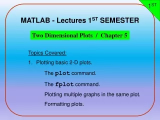
1ST MATLAB - Lectures 1ST SEMESTER Two Dimensional Plots / Chapter 5 Topics Covered: • Plotting basic 2-D plots. The plot command. The fplot command. Plotting multiple graphs in the same plot. Formatting plots.
1ST MAKING X-Y PLOTS MATLAB has many functions and commands that can be used to create various types of plots. In our class we will only create two dimensional x – y plots.
1ST EXAMPLE OF A 2-D PLOT Legend Plot title y axis label Text Tick-mark Data symbol x axis label Tick-mark label
1ST LAB1 TWO-DIMENSIONAL plot() COMMAND The basic 2-D plot command is: plot(x,y) where x is a vector (one dimensional array), and y is a vector. Both vectors must have the same number of elements. • The plot command creates a single curve with the x values on the abscissa (horizontal axis) and the y values on the ordinate (vertical axis). • The curve is made from segments of lines that connect the points that are defined by the x and y coordinates of the elements in the two vectors.
1ST CREATING THE X AND Y VECTORS • If data is given, the information is entered as the elements of the vectors x and y. • If the values of y are determined by a function from the values of x, than a vector x is created first, and then the values of y are calculated for each value of x. The spacing (difference) between the elements of x must be such that the plotted curve will show the details of the function.
x 1 2 3 5 7 7.5 8 10 y 2 6.5 7 7 5.5 4 6 8 1ST PLOT OF GIVEN DATA Given data: A plot can be created by the commands shown below. This can be done in the Command Window, or by writing and then running a script file. >> x=[1 2 3 5 7 7.5 8 10]; >> y=[2 6.5 7 7 5.5 4 6 8]; >> plot(x,y) Once the plot command is executed, the Figure Window opens with the following plot.
1ST PLOT OF GIVEN DATA
plot(x,y,’line specifiers’) 1ST LAB2 LINE SPECIFIERS IN THE plot() COMMAND Line specifiers can be added in the plot command to: • Specify the style of the line. • Specify the color of the line. • Specify the type of the markers (if markers are desired).
plot(x,y,‘line specifiers’) 1ST LINE SPECIFIERS IN THE plot() COMMAND Line Specifier Line Specifier Marker Specifier Style Color Type Solid - red r plus sign + dotted : green g circle o dashed -- blue b asterisk * dash-dot -. Cyan c point . magenta m square s yellow y diamond d black k
1ST LINE SPECIFIERS IN THE plot() COMMAND • The specifiers are typed inside the plot() command as strings. • Within the string the specifiers can be typed in any order. • The specifiers are optional. This means that none, one, two, or all the three can be included in a command. EXAMPLES: plot(x,y) A solid blue line connects the points with no markers. plot(x,y,’r’) A solid red line connects the points with no markers. plot(x,y,’--y’) A yellow dashed line connects the points. plot(x,y,’*’) The points are marked with * (no line between the points.) plot(x,y,’g:d’) A green dotted line connects the points which are marked with diamond markers.
Year 1988 1989 1990 1991 1992 1993 1994 Sales (M) 127 130 136 145 158 178 211 Line Specifiers: dashed red line and asterisk markers. 1ST PLOT OF GIVEN DATA USING LINE SPECIFIERS IN THE plot() COMMAND >> year = [1988:1:1994]; >> sales = [127, 130, 136, 145, 158, 178, 211]; >> plot(year,sales,'--r*')
1ST PLOT OF GIVEN DATA USING LINE SPECIFIERS IN THE plot() COMMAND Dashed red line and asterisk markers.
1ST CREATING A PLOT OF A FUNCTION Consider: A script file for plotting the function is: % A script file that creates a plot of % the function: 3.5^(-0.5x)*cos(6*x) x = [-2:0.01:4]; y = 3.5.^(-0.5*x).*cos(6*x); plot(x,y) Creating a vector with spacing of 0.01. Calculating a value of y for each x. Once the plot command is executed, the Figure Window opens with the following plot.
1ST A PLOT OF A FUNCTION
1ST CREATING A PLOT OF A FUNCTION If the vector x is created with large spacing, the graph is not accurate. Below is the previous plot with spacing of 0.3. x = [-2:0.3:4]; y = 3.5.^(-0.5*x).*cos(6*x); plot(x,y)
1ST THE fplot COMMAND LAB 3 The fplot command can be used to plot a function with the form: y = f(x) fplot(‘function’,limits) • The function is typed in as a string. • The limits is a vector with the domain of x, and optionally with limits of the y axis: [xmin,xmax] or [xmin,xmax,ymin,ymax] • Line specifiers can be added.
1ST PLOT OF A FUNCTION WITH THE fplot() COMMAND A plot of: >> fplot('x^2 + 4 * sin(2*x) - 1', [-3 3])
1ST PLOTTING MULTIPLE GRAPHS IN THE SAME PLOT Plotting two (or more) graphs in one plot: • Using the plot command. 2. Using the holdon, hold off commands.
1ST USING THE plot() COMMAND TO PLOT MULTIPLE GRAPHS IN THE SAME PLOT plot(x,y,u,v,t,h) Plots three graphs in the same plot: y versus x, v versus u, and h versus t. • By default, MATLAB makes the curves in different colors. • Additional curves can be added. • The curves can have a specific style by adding specifiers after each pair, for example: plot(x,y,’-b’,u,v,’—r’,t,h,’g:’)
Plot of the function, and its first and second derivatives, for , all in the same plot. 1ST USING THE plot() COMMAND TO PLOT MULTIPLE GRAPHS IN THE SAME PLOT x = [-2:0.01:4]; y = 3*x.^3-26*x+6; yd = 9*x.^2-26; ydd = 18*x; plot(x,y,'-b',x,yd,'--r',x,ydd,':k') vector x with the domain of the function. Vector y with the function value at each x. Vector yd with values of the first derivative. Vector ydd with values of the second derivative. Create three graphs, y vs. x (solid blue line), yd vs. x (dashed red line), and ydd vs. x (dotted black line) in the same figure.
1ST USING THE plot() COMMAND TO PLOT MULTIPLE GRAPHS IN THE SAME PLOT
1ST USING THE hold on, hold off, COMMANDS TO PLOT MULTIPLE GRAPHS IN THE SAME PLOT hold on Holds the current plot and all axis properties so that subsequent plot commands add to the existing plot. hold off Returns to the default mode whereby plot commands erase the previous plots and reset all axis properties before drawing new plots. This method is useful when all the information (vectors) used for the plotting is not available a the same time.
Plot of the function, and its first and second derivatives, for all in the same plot. 1ST USING THE hold on, hold off, COMMANDS TO PLOT MULTIPLE GRAPHS IN THE SAME PLOT x = [-2:0.01:4]; y = 3*x.^3-26*x+6; yd = 9*x.^2-26; ydd = 18*x; plot(x,y,'-b') hold on plot(x,yd,'--r') plot(x,ydd,':k') hold off First graph is created. Two more graphs are created.
1ST EXAMPLE OF A FORMATTED 2-D PLOT Plot title Legend y axis label Text Tick-mark Data symbol x axis label Tick-mark label
1ST LAB 4 FORMATTING PLOTS A plot can be formatted to have a required appearance. With formatting you can: • Add title to the plot. • Add labels to axes. • Change range of the axes. • Add legend. • Add text blocks. • Add grid.
1ST FORMATTING PLOTS There are two methods to format a plot: • Formatting commands. In this method commands, that make changes or additions to the plot, are entered after the plot() command. This can be done in the Command Window, or as part of a program in a script file. • Formatting the plot interactively in the Figure Window. In this method the plot is formatted by clicking on the plot and using the menu to make changes or add details.
1ST FORMATTING COMMANDS title(‘string’) Adds the string as a title at the top of the plot. xlabel(‘string’) Adds the string as a label to the x-axis. ylabel(‘string’) Adds the string as a label to the y-axis. axis([xmin xmax ymin ymax]) Sets the minimum and maximum limits of the x- and y-axes.
1ST FORMATTING COMMANDS legend(‘string1’,’string2’,’string3’) Creates a legend using the strings to label various curves (when several curves are in one plot). The location of the legend is specified by the mouse. text(x,y,’string’) Places the string (text) on the plot at coordinate x,y relative to the plot axes. gtext(‘string’) Places the string (text) on the plot. When the command executes the figure window pops and the text location is clicked with the mouse.
1ST EXAMPLE OF A FORMATTED PLOT Below is a script file of the formatted light intensity plot (2nd slide). (Some of the formatting options were not covered in the lectures, but are described in the book) x=[10:0.1:22]; y=95000./x.^2; xd=[10:2:22]; yd=[950 640 460 340 250 180 140]; plot(x,y,'-','LineWidth',1.0) hold on plot(xd,yd,'ro--','linewidth',1.0,'markersize',10) hold off Creating vector x for plotting the theoretical curve. Creating vector y for plotting the theoretical curve. Creating a vector with coordinates of data points. Creating a vector with light intensity from data.
Creating text. 1ST EXAMPLE OF A FORMATTED PLOT Formatting of the light intensity plot (cont.) xlabel('DISTANCE (cm)') ylabel('INTENSITY (lux)') title('\fontname{Arial}Light Intensity as a Function of Distance','FontSize',14) axis([8 24 0 1200]) text(14,700,'Comparison between theory and experiment.','EdgeColor','r','LineWidth',2) legend('Theory','Experiment',0) Labels for the axes. Title for the plot. Setting limits of the axes. Creating a legend. The plot that is obtained is shown again in the next slide.
1ST EXAMPLE OF A FORMATTED PLOT
Use Figure, Axes, and Current Object-Properties in the Edit menu 1ST FORMATTING A PLOT IN THE FIGURE WINDOW Once a figure window is open, the figure can be formatted interactively. Use the insert menu to Click here to start the plot edit mode.
1ST Adding Titles to Graphs • You can add a title to a graph in several ways, described in the following sections. Using the Title Option on the Insert Menu To add a title to a graph using the Insert menu: 1.Click the Insert menu in the figure menu bar and choose Title. A text entry box opens at the top of the axes. 2. Enter the text of the label.
1ST Using the Property Editor to Add a Title To add a title to a graph using the Property Editor :- • Start plot editing mode by selecting Edit Plot from the figure Tools menu. • Double-click an empty region of the axes in the graph. This starts the Property Editor. You can also start the Property Editor by right-clicking on the axes and selecting Show Property Editor from the context menu or by selecting Property Editor from the View menu. • Type the text of your title in the Title text entry box.
1ST You can change the font, font style, position, and many other aspects of the title format. • To move the title, select the text and drag it to the desired position. • To edit the text, double-click the title and type new characters. • To change the font and other text properties, select the title and right-click to display the context menu
1ST Adding grid to the plot • It is useful to add grid to the plot by using grid command after use plot command • grid on % to open grid • grid off % to close grid x=[10:0.1:22]; y=95000./x.^2; plot(x,y,'-','LineWidth',1.0) grid on xlabel('DISTANCE (cm)') ylabel('INTENSITY (lux)') title('\fontname{Arial}Fig(1):Light Intensity as a Function of Distance','FontSize',14)
1ST WE OBTAIN THE FOLLOWING FIGURE :-
1ST LAB 5 Creat Figure Graphics Object MATLAB creates a new window whose characteristics are controlled by default figure properties (both factory installed and user defined ) and properties specified as argument figure(h) where h is an integer ,creates a new figure window ,or makes figure h the current figure .Subsequent plots are drawn in the current figure . h is called the handle of the figure .
1ST clc clear all clf % clf clears the current figure window. It also resets all % properties associated with the axes ,such as the hold state % and the axis state . x = 0:pi/40:4*pi; figure(1) % plot with first properties plot(x,sin(x),’r*’) figure(2) % plot with second properties plot(x,cos(x),’mo’) Ex:-
1ST We will get two separated figures in two windows :-
1ST You can show a number of plots in the same figure window with the subplot function The general Syntax subplot (m, n , p) where :- m : number of rows . n : number of columns . p : number of matrix which occupy the figure . divides the figure windows into m x n small sets of axes , and selects the pth set for the current plot (numbered by row from the left of the top row ). Multiple Plots In A Figure : subplot
1ST clc clear all clf x = 0:0.1:10; y = sin (x); z = cos (x); subplot (1,2,1) plot(x,y,’r*’) grid on subplot (1,2,2) plot(x,z,’mo’) grid on Ex:-
1ST clc, clear all, clf x = 0:0.1:10; y = sin (x); z = cos (x); v = exp(x) subplot (3,3,[1 2 3 4 5 6 ]) plot(x,y,’r*’) grid on subplot (337) plot(x,z,’mo’) grid on subplot(339) plot(x,v) grid on