It’s a kind of MAGIC! Come i raggi gamma ad altissima energia diventano segnale

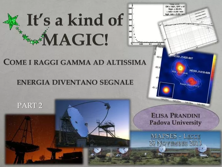
1. It’s a kind of MAGIC!Come iraggi gamma ad altissimaenergiadiventanosegnale Elisa Prandini Padova University MAPSES – Lecce 23 November 2011 PART 2

2. Summary • Intro: VHE g-rays Astrophysics • Observation Technique • Instruments and data taking • From raw data to shower images • Background Rejection • Signal extraction • Results: • Sky Maps • Integral and differential fluxes

3. Steps of the Analysis of CT data Pixel signal extraction Raw signal Image cleaning Image parameterization Cleaned signal Stereo- reconstruction Event parameter reconst Detection Background rejection Background estimation Source detection Sky maps Spectrum Spectrum / light curve Spectrum Unfolding

4. Characterization of the events Once we have obtained the shower images, the next step is to obtain the characteristics of the primary particle which originated the shower • Nature of the particle (Background rejection) • Primary Direction • Primary Energy

5. Random Forest Reloaded

6. Random Forests Based on Monte Carlo Simulation + real data How it works: The growing of a tree • elements: • - parameters (~10) • trees (100) • In each tree: • nodes • Possible parameters in each node (trials, ~3)  RANDOM • best separator and value per node (via Gini index) • final node size (1-5) • each event is classified! training this is a tree Application to real data: - We apply each tree ( from training) to them - Each event is univocally classified (with a local hadronness)  Final hadronness is an average among all the values!

7. Primary direction

8. Primary direction • The ellipse major axis points to the center of the camera • With many telescopes: • The intersection of the axes is related to the incoming direction Helpful to “detect the signal”

9. The incoming direction

10. Reconstruction of the incoming direction Geometrical reconstruction: for more than 1 telescope Efficient for δ 30 deg In Plan ┴ direction M1 M2 Impact parameter Δδ Reconstructed direction Reconstructed core impact point M1 M2 Monte Carlo independent

11. Energy Reconstruction

12. Energy reconstruction Basic fact: Energy ~ Image size Methods: • A parameterization: Energy = f(size, impact, zenith,…) • Look-up tables • Optimized decision trees (Random Forest) Based on Monte Carlo Simulation

13. Energy reconstruction Energyresolution: 20% at 100 GeV, downto 15% around 1 TeV Energy Resolution: E(est) - E(true) / E(true) Energy Bias: E(est) - E(true) / E(est) Big bias @ low energies. Solved with unfolding Estimated with Monte Carlo (Gammas)

14. Signal Extraction

15. What is the aim of our analysis? • Populate the VHE sky • Localize the emission • Characterize the emission • Energy • Time Detection of the Signal Sky Map Spectrum Lightcurve

16. The analysis File  Set of Events Event  Set of Parameters characterizing the shower Remember: event  is a shower (induced by a CR) • Data acquisition • Calibration • Image cleaning and Hillas Parameters calculation • Hadronness and energy reconstruction Former steps

17. Characteristics of a g-like event Therefore if we plot the parameter related to the reconstructed incoming direction, the gamma-like events will have it close to the telescopes pointing direction • To discriminate gamma-ray induced images from hadrons induced images, we use the square of the parameter q, the angle between the pointing direction (camera center) and the (reconstructed) incoming direction. • And what about the hadrons? • They are randomly distributed!

18. Detection: the Theta2 plot! • Where is the signal???

19. ? We have a problem… The number of background events is ~ 104 times the number of gamma Events We have to reduce the number of bkg events: • HADRONNESS PARAMETER! • We apply a cut and reject the events that are likely hadrons (MC data)

20. The Detection • Now we are ready to perform our detection plot (also called theta-square plot) VERITAS Collaboration, V. A. Acciari et al, ApJ 715 (2010) L49 Source data “Signal” Background data

21. The Background • We need a background in order to estimate the signal • Old technique: observe the source (ON data) and a region of the sky with the same characteristics but without a source (OFF data) PROBLEMS- time consuming! - different observations conditions (weather, hardware) • SOLUTION: find an observing mode which allows to collect ON and OFF data simultaneously! • Wobble mode: the telescopes point to a region 0.4 deg offset from the source (and the background can be extracted)

22. The Detection • Some theta2 plots: VERITAS Collaboration, V. A. Acciari et al, ApJ 715 (2010) L49 H.E.S.S. Collaboration, F. Aharonian et al. A&A 442 (2005) 177-183 Not always there is a detection of course…

23. The Significance • significance is a measure of the likelihood that pure background fluctuations have produced the observed excess (i.e., assuming no signal) • The common rule is that a source is detected if the significance of the signal exceeds 5 sigma! • We need a tool to say if our observation is physically relevant • We use the significance of the signal Li, T., and Ma, Y. 1983, ApJ, 272, 317

24. Mkn 180 MAGIC Examples • A five sigma signal • A four sigma signal • A 10 sigma signal PKS 1222+21 MAGIC PG 1553+113 H.E.S.S.

25. Standard Example: the Crab Nebula • MAGIC observations of the Crab Nebula: E>300 GeV 60 GeV < E < 100 GeV The energy range considered! • WHICH IS THE DIFFERENCE?

26. Images and Energy At low energies the characterization of a gamma-like is much more difficult!!!

27. Therefore: • The data analysis of IACTs telescopes is non trivial… • The first result to look for is a signal (is there a gamma ray source or not?): • The tool is the theta2 plot, a plot of the parameter theta2, that discriminates between hadrons (our background) and gamma-rays induced showers using the incoming direction • The signal is quantified through its Significance: • < 5 sigma  no signal or more statistics needed • > 5 sigma  there is a signal! The analysis can continue

28. Physical Results Sky Maps

29. Second step: the localization • Important: in general IACTs don’t operate in scan mode but in pointing mode! • Moreover our resolution is… ~ 0.1 degrees • Extended sources: are galactic and very large regions • Extragalactic objects, for the moment, are point-like! In order to localize the emission, we perform the so-called sky map, that is a bi-dimensional map of the reconstructed incoming directions of the primary gamma rays

30. The sky map • For each event we reconstruct the incoming direction • Is the same parameter that we have used in the detection plot! • The background is modeled • Remember: our PSF is ~ 0.1 degree… • We use it: • As a check tool • In few cases: extended emission or multiple sources in the field

31. Example: the Crab Nebula Find the difference!

32. Example: the Crab Nebula The angular resolution is strictly related to the Energy range!

33. Extended sources • Some galactic sources are extended enough to be mapped nicely at TeV energies • SNR HESS J1731-347 • Very interesting studies on acceleration sites! H.E.S.S. collaboration, A. Abramowski et al. A&A 531 (2011) A81

34. NGC 1275 region • Clear signal from the head tail RG IC 310 at E > 400 GeV • And below this energy? E > 400 GeV • If we go down to 150 GeV, a signal from the RG NGC 1275 becomes significant! E > 150 GeV

35. The galactic scan HESS Coll. ICRC 2009 Proceedings

36. So, in the lucky case: • We have detected a significant signal • We have checked that the emission is coming from the direction that we expect (if not, go back to point 1, changing the true source position) • Now? • Spectrum • Light curve

37. Physical Results The Spectrum

38. The differential energy spectrum • The spectrum is essential in our study • Allows the characterization of the emission • A comparison is possible (also between different experiments and energy thresholds!) • What is it? The number of VHE photons per area and time VERITAS Coll. APJ Letters, 709, L163-L167 (2010)

39. Definitions • -ray flux: rate of -rays per unit area ( to their direction) • units: [L-2][T-1] (e.g. cm-2 s-1) • Needed ingredients: a number of -rays, a collection area and an observation time Related concepts: • Differential energy spectrum: flux per interval in -ray energy (cm-2 s-1 TeV-1) • Integral flux: integrated in a given energy range (cm-2 s-1), e.g. : • Light curve: time evolution of integral flux:  vs. t Courtesy of A. Moralejo

40. Differential energy spectrum:the observables Number of detected -rays: obtained from the observed excess Effective collection area Estimated energy of the events Effective observation time: not equal to the elapsed time!

41. Number of g-rays per energy • We have a “discretization” dN/dE becomes the number of excess per energy interval • How do we estimate this quantity? Through the theta2 plot (per energy interval)!

42. probability of observing n events in time t, given event rate  probability that the next event comes after time t Effective observation time • The effective observation time is not equal to the elapsed time between the beginning and end of the observations: • there may be gaps in the data taking (e.g. between runs) • there is a dead time after the recording of each event • Useful quantity: t, the time difference between the arrival time of an event and the next one • In a Poisson process, t follows an exponential Courtesy of A. Moralejo

43. Calculation of effective observation time • Distribution of the time differences: In case of fixed dead time d, the distribution is still exponential with slope  The true rate of events  (i.e. before the detector) can be obtained from an exponential fit to the distribution And teff = Nd,0 / Courtesy of A. Moralejo

44. Example effective time l slope N  intercept And teff = Nd,0 / Log scale!

45. Effective Area • Order of magnitude? Aeff ~105 m2 Estimated from MC (gamma) data!

46. Effective Area • Order of magnitude Aeff ~105 m2 • It’s roughly the Cherenkov light pool • Depends on the Zenith angle of the observations: We estimate it with MC data

47. Differential energy spectra • Numbers of bins is of course variable and set by the analyzer • Errors are larger at high energies… why? • Usually fitted with power laws

48. The unfolding • Before publishing our spectrum, there is still one thing that we can do: • Use the MC data to calculate the errors that we perform and apply a correction to the data • limited acceptance and finite resolution • systematic distortions • reconstructed energy is not true energy! How? With a matrix (correlation matrix) correlating the true Energy (from simulations) to the reconstructed Energy (estimated through RF)

49. Crab Nebula Spectrum …and SED

50. Other examples • Extremely variable objects • Extremely distant objects (z=0.536)