Download

1 / 38
380 likes | 483 Views
Explore the basics of probability in classification using a Naïve Bayes Classifier. Learn about generative and discriminative models, probability calculations, classifier methods, and practical examples. Understand the Naïve Bayes algorithm and its application in classification tasks. Dive into issues related to Naïve Bayes, such as the violation of independence assumptions and zero conditional probability problems.

E N D
QUIZZ: Probability Basics • Quiz: We have two six-sided dice. When they are rolled, it could end up with the following occurrence: (A) dice 1 lands on side “3”, (B) dice 2 lands on side “1”, and (C) Two dice sum to eight. Answer the following questions:
Probabilistic Classification • Establishing a probabilistic model for classification • Discriminative model What is a discriminative Probabilistic Classifier? • Example • C1 – benign mole • C2 - cancer Discriminative Probabilistic Classifier
Probabilistic Classification • Establishing a probabilistic model for classification (cont.) • Generative model Probability that this fruit is an orange Probability that this fruit is an apple Generative Probabilistic Model for Class L Generative Probabilistic Model for Class 1 Generative Probabilistic Model for Class 2
Background: Methods to create classifiers • There are three methods to establish a classifier a) Model a classification rule directly Examples: k-NN, decision trees, perceptron, SVM b) Model the probability of class memberships given input data Example: Perceptron with the cross-entropy cost c) Make a probabilistic model of data within each class Examples: Naive Bayes, model based classifiers • a) and b) are examples of discriminative classification • c) is an example of generative classification • b) and c) are both examples of probabilistic classification GOOD NEWS: You can create your own hardware/software classifiers!
Probability Basics • We defined prior, conditional and joint probability for random variables • Prior probability: • Conditional probability: • Joint probability: • Relationship: • Independence: • Bayesian Rule
Method: Probabilistic Classification with MAP • MAP classification rule • MAP: Maximum APosterior • Assign x to c* if • Method of Generative classification with the MAP rule • Apply Bayesian rule to convert them into posterior probabilities • Then apply the MAP rule We use this rule in many applications
For a class, the previous generative model can be decomposed by n generative models of a single input. Naïve Bayes • Bayes classification • Difficulty: learning the joint probability • Naïve Bayes classification • Assumption that all input attributes are conditionally independent! • MAP classification rule: for Product of individual probabilities
Naïve Bayes Algorithm • Naïve Bayes Algorithm (for discrete input attributes) has two phases • 1. Learning Phase: Given a training set S, • Output: conditional probability tables; for elements • 2. Test Phase: Given an unknown instance , • Look up tables to assign the label c* to X’ if Learning is easy, just create probability tables. Classification is easy, just multiply probabilities
Tennis Example • Example: Play Tennis
The learning phase for tennis example P(Play=Yes) = 9/14 P(Play=No) = 5/14 We have four variables, we calculate for each we calculate the conditional probability table
Formulation of a Classification Problem • Given the data as found in last slide: • Find for a new point in space (vector of values) to which group it belongs (classify)
The test phase for the tennis example • Test Phase • Given a new instance of variable values, • x’=(Outlook=Sunny, Temperature=Cool, Humidity=High, Wind=Strong) • Given calculated Look up tables • Use the MAP rule to calculate Yes or No P(Outlook=Sunny|Play=Yes) = 2/9 P(Temperature=Cool|Play=Yes) = 3/9 P(Huminity=High|Play=Yes) = 3/9 P(Wind=Strong|Play=Yes) = 3/9 P(Play=Yes) = 9/14 P(Outlook=Sunny|Play=No) = 3/5 P(Temperature=Cool|Play==No) = 1/5 P(Huminity=High|Play=No) = 4/5 P(Wind=Strong|Play=No) = 3/5 P(Play=No) = 5/14 P(Yes|x’): [P(Sunny|Yes)P(Cool|Yes)P(High|Yes)P(Strong|Yes)]P(Play=Yes) = 0.0053 P(No|x’): [P(Sunny|No) P(Cool|No)P(High|No)P(Strong|No)]P(Play=No) = 0.0206 Given the fact P(Yes|x’) < P(No|x’), we label x’ to be “No”.
Issues Relevant to Naïve Bayes • Violation of Independence Assumption • Zero conditional probability Problem
Issues Relevant to Naïve Bayes First Issue • Violation of Independence Assumption • For many real world tasks, • Nevertheless, naïve Bayes works surprisingly well anyway! Events are correlated
Issues Relevant to Naïve Bayes Second Issue • Zero conditional probability Problem • Such problem exists when no example contains the attribute value • In this circumstance, during test • For a remedy, conditional probabilities are estimated with
Another Problem: Continuous-valued Input Attributes • What to do in such a case? • Numberless values for an attribute • Conditional probability is then modeled with the normal distribution • Learning Phase: • Output: normal distributions and • Test Phase: • Calculate conditional probabilities with all the normal distributions • Apply the MAP rule to make a decision
Naïve Bayes Training • Now that we’ve decided to use a Naïve Bayes classifier, we need to train it with some data:
Naïve Bayes Training • Training in Naïve Bayes is easy: • –Estimate P(Y=v) as the fraction of records with Y=v • Estimate P(Xi=u|Y=v) as the fraction of records with Y=v for which Xi=u
Naïve Bayes Training • In practice, some of these counts can be zero • Fix this by adding “virtual” counts: • This is called Smoothing
Naïve Bayes Training • For binary digits, training amounts to averaging all of the training fives together and all of the training sixes together.
Conclusion on classifiers • Naïve Bayes is based on the independence assumption • Training is very easy and fast; just requiring considering each attribute in each class separately • Test is straightforward; just looking up tables or calculating conditional probabilities with normal distributions • Naïve Bayes is a popular generative classifier model • Performance of naïve Bayes is competitive to most of state-of-the-art classifiers even if in presence of violatingthe independence assumption • It has many successful applications, e.g., spam mail filtering • A good candidate of a base learner in ensemble learning • Apart from classification, naïve Bayes can do more…
https://www.datasciencecentral.com/profiles/blogs/naive-bayes-in-one-picture-1https://www.datasciencecentral.com/profiles/blogs/naive-bayes-in-one-picture-1
R Example (http://uc-r.github.io/naive_bayes) • To illustrate the naïve Bayes classifier we will use the attrition data that has been included in the rsample package. The goal is to predict employee attrition. library(rsample) # data splitting library(dplyr) # data transformation library(ggplot2) # data visualization library(caret) # implementing with caret library(h2o) # implementing with h2o
# convert some numeric variables to factors attrition <- attrition %>% mutate( JobLevel = factor(JobLevel), StockOptionLevel = factor(StockOptionLevel), TrainingTimesLastYear = factor(TrainingTimesLastYear) ) # Create training (70%) and test (30%) sets for the attrition data. # Use set.seed for reproducibility set.seed(123) split <- initial_split(attrition, prop = .7, strata = "Attrition") train <- training(split) test <- testing(split) # distribution of Attrition rates across train & test set table(train$Attrition) %>% prop.table() No Yes 0.838835 0.161165 table(test$Attrition) %>% prop.table() No Yes 0.8386364 0.1613636
With naïve Bayes, we assume that the predictor variables are conditionally independent of one another given the response value. This is an extremely strong assumption. We can see quickly that our attrition data violates this as we have several moderately to strongly correlated variables. library(corrplot) train %>% filter(Attrition == "Yes") %>% select_if(is.numeric) %>% cor() %>% corrplot::corrplot()
However, by making this assumption we can simplify our calculation such that the posterior probability is simply the product of the probability distribution for each individual variable conditioned on the response category. • For categorical variables, this computation is quite simple as you just use the frequencies from the data. However, when including continuous predictor variables often an assumption of normality is made so that we can use the probability from the variable’s probability density function. If we pick a handful of our numeric features we quickly see assumption of normality is not always fair. train %>% select(Age, DailyRate, DistanceFromHome, HourlyRate, MonthlyIncome, MonthlyRate) %>% gather(metric, value) %>% ggplot(aes(value, fill = metric)) + geom_density(show.legend = FALSE) + facet_wrap(~ metric, scales = "free")
Some numeric features may be normalized with a Box-Cox transformation; however, we can also use non-parametric kernel density estimators to try get a more accurate representation of continuous variable probabilities. Ultimately, transforming the distributions and selecting an estimator is part of the modeling development and tuning process. • Laplace Smoother • We run into a serious problem when new data includes a feature value that never occurs for one or more levels of a response class. What results is P(xi|Ck)=0 for this individual feature and this zero will ripple through the entire multiplication of all features and will always force the posterior probability to be zero for that class. • A solution to this problem involves using the Laplace smoother. The Laplace smoother adds a small number to each of the counts in the frequencies for each feature, which ensures that each feature has a nonzero probability of occurring for each class. Typically, a value of one to two for the Laplace smoother is sufficient, but this is a tuning parameter to incorporate and optimize with cross validation.
First, we apply a naïve Bayes model with 10-fold cross validation, which gets 83% accuracy. Considering about 83% of our observations in our training set do not attrit, our overall accuracy is no better than if we just predicted “No” attrition for every observation. • There are several packages to apply naïve Bayes (i.e. e1071, klaR, naivebayes, bnclassify). library(klaR) # create response and feature data features <- setdiff(names(train), "Attrition") x <- train[, features] y <- train$Attrition # set up 10-fold cross validation procedure train_control <- trainControl( method = "cv", number = 10 ) # train model nb.m1 <- train( x = x, y = y, method = "nb", trControl = train_control ) # results confusionMatrix(nb.m1) Cross-Validated (10 fold) Confusion Matrix (entries are percentual average cell counts across resamples) Reference Prediction No Yes No 75.2 8.1 Yes 8.6 8.1 Accuracy (average) : 0.833
We can tune the few hyperparameters that a naïve Bayes model has. • Usekernel parameter allows us to use a kernel density estimate for continuous variables versus a guassian density estimate, • adjust allows us to adjust the bandwidth of the kernel density (larger numbers mean more flexible density estimate), • fL allows us to incorporate the Laplace smoother. • If we just tuned our model with the above parameters we are able to lift our accuracy to 85%; however, by incorporating some preprocessing of our features (normalize with Box Cox, standardize with center-scaling, and reducing with PCA) we actually get about another 2% lift in our accuracy.
# set up tuning grid search_grid <- expand.grid( usekernel = c(TRUE, FALSE), fL = 0:5, adjust = seq(0, 5, by = 1) ) # train model nb.m2 <- train( x = x, y = y, method = "nb", trControl = train_control, tuneGrid = search_grid, preProc = c("BoxCox", "center", "scale", "pca") ) # top 5 modesl nb.m2$results %>% top_n(5, wt = Accuracy) %>% arrange(desc(Accuracy)) usekernelfL adjust Accuracy Kappa AccuracySDKappaSD 1 TRUE 1 3 0.8738671 0.4249084 0.02902693 0.1516638 2 TRUE 2 3 0.8690688 0.4555071 0.03590654 0.1593024 3 TRUE 3 4 0.8690408 0.4404052 0.03069306 0.1545643 4 TRUE 0 2 0.8680792 0.4177358 0.03513233 0.1592905 5 TRUE 3 5 0.8680133 0.3697180 0.02361187 0.1284321
# plot search grid results plot(nb.m2)
# results for best model confusionMatrix(nb.m2) Cross-Validated (10 fold) Confusion Matrix (entries are percentual average cell counts across resamples) Reference Prediction No Yes No 81.2 9.9 Yes 2.7 6.2 Accuracy (average) : 0.8738 We can assess the accuracy on our final holdout test set. pred <- predict(nb.m2, newdata = test) confusionMatrix(pred, test$Attrition) Confusion Matrix and Statistics Reference Prediction No Yes No 349 41 Yes 20 30 Accuracy : 0.8614 95% CI : (0.8255, 0.8923) No Information Rate : 0.8386 P-Value [Acc > NIR] : 0.10756 Kappa : 0.4183 Mcnemar's Test P-Value : 0.01045 Sensitivity : 0.9458 Specificity : 0.4225 PosPred Value : 0.8949 NegPred Value : 0.6000 Prevalence : 0.8386 Detection Rate : 0.7932 Detection Prevalence : 0.8864 Balanced Accuracy : 0.6842 'Positive' Class : No
Some Other Sources • https://web.stanford.edu/class/cs124/lec/naivebayes.pptx • https://cse.sc.edu/~rose/587/PPT/NaiveBayes.ppt • http://studentnet.cs.manchester.ac.uk/ugt/COMP24111/materials/slides/Naive-Bayes.ppt • http://www.cs.kent.edu/~jin/DM11/Naive-Bayes.ppt