Testing Surface Area
Discover groundbreaking joint work by Ryan O’Donnell and collaborators on surface area testing in multiple dimensions. This nonadaptive algorithm allows efficient queries to determine shape properties. No assumptions needed!


Testing Surface Area
E N D
Presentation Transcript
Testing Surface Area Ryan O’Donnell Carnegie Mellon & Boğaziçi University joint work with Pravesh Kothari(UT Austin),Amir Nayyeri (Oregon), Chenggang Wu (Tsinghua)
In 2 dimensions… BTW: This is one shape,that happens to bedisconnected “surface area” is called “perimeter”
In 1 dimension… BTW: This is one shape,that happens to bedisconnected “surface area” equals “# of endpoints” = “2 × # of intervals”
Our Theorem Given S, ϵ, and query access to F ⊂ [0,1]n, there’s an O(1/ϵ)-query (nonadaptive) algorithm s.t.: vol(F∆G) > ϵ • Says YES whp if perim(F) ≤ S; • Says NO whp if F is ϵ-far from all Gwith perim(G) ≤1.28S.
Our Theorem Given S, ϵ, and query access to F ⊂ [0,1]n, there’s an O(1/ϵ)-query (nonadaptive) algorithm s.t.: • Says YES whp if perim(F) ≤ S; • Says NO whp if F is ϵ-far from all Gwith perim(G) ≤1.28S. No Curse Of Dimensionality! No assumptions about F!
Our Theorem Given S, ϵ, and query access to F ⊂ [0,1]n, there’s an O(1/ϵ) -query (nonadaptive) algorithm s.t.: 1 ϵδ2.5 • Says YES whp if perim(F) ≤ S; • Says NO whp if F is ϵ-far from all Gwith perim(G) ≤(κn+δ)S.
Prior work who dim. queries approx factor κ [KR98] 1 O(1/ϵ) 1/ϵ O(1/ϵ4) [BBBY12] 1 1 O(1/ϵ3.5) 1 1 [KNOW14] < 1.28 ∀nany 1+δ if n=1 O(1/ϵ) n any 1+δ [Nee14] n O(1/ϵ)
Prior work who dim. queries approx factor κ [KR98] 1 O(1/ϵ) 1/ϵ O(1/ϵ4) [BBBY12] 1 1 O(1/ϵ3.5) 1 1 [KNOW14] < 1.28 ∀nany 1+δ if n=1 Remark: We obtained same results inGaussian space. So did Neeman. O(1/ϵ) n any 1+δ [Nee14] n O(1/ϵ)
Property Testing framework is necessary Theorem [BNN06]: If F ⊂ [0,1]n promised to be convex, can estimate perim(F) to factor 1+δ whp using poly(n/δ) queries. No “ϵ-far” stuff. We don’t assume convexity, curvature bounds,connectedness — nothing.
Soundness theorem challenge:Cut string, smooth side, fill in holes.
Algorithm: Buffon’s Needle Crofton Formula. Let F ⊂ [0,1]n Pick x ~ ℝn/ℤn uniformly. Pick y ~ Bλ(x). Line segment xy called “the needle”. Then… ℝn/ℤn. E[ #(xy∩∂F) ] = cn ·λ· perim(F) y x F
Algorithm: Buffon’s Needle Crofton Formula. Let F ⊂ [0,1]n Pick x ~ ℝn/ℤn uniformly. Pick y ~ Bλ(x). Line segment xy called “the needle”. Then… explicit dimension-dependent constant, Θ(n–1/2) ℝn/ℤn. E[ #(xy∩∂F) ] = cn ·λ· perim(F) y x F
The “Noise Sensitivity” of F: NSF(λ) := Pr[ 1F(x)≠1F(y) ] = E[ 1{x∈F, y∉F, or vice versa} ] ≤ E[ #(xy∩∂F) ] = cn ·λ· perim(F) y x F
Algorithm and Completeness Recall: NSF(λ) = Pr [ 1F(x) ≠ 1F(y) ] x ~ ℝn/ℤn y ~ Bλ(x)’ ≤ cn · λ· perim(F) 0. Given S, ϵ, set λ such that ϵ = .01 · cn · λ· S. 1. Empirically estimate NSF(λ). 2. Say YES iff ≤ (1+δ) · cn · λ· S. Query complexity, Completeness: ✔
Soundness? Recall: NSF(λ) = Pr [ 1F(x) ≠ 1F(y) ] x ~ ℝn/ℤn y ~ Bλ(x)’ ≤ cn · λ· perim(F) 0. Given S, ϵ, set λ such that ϵ = .01 · cn · λ· S. 1. Empirically estimate NSF(λ). 2. Say YES iff ≤ (1+δ) · cn · λ· S. Query complexity, Completeness: ✔
Soundness? Recall: NSF(λ) = Pr [ 1F(x) ≠ 1F(y) ] x ~ ℝn/ℤn y ~ Bλ(x)’ ≤ cn · λ· perim(F) Q: If NSF(λ) ≤ cn · λ· S, is perim(F) ≾ S? Q: I.e., is perim(F) ≾ (cnλ)–1 · NSF(λ) always? A: Not necessarily. (F may “wiggle at a scale ≪λ”.) Q: Is F at least close to some G with perim(G) ≾ (cnλ)–1 · NSF(λ) ? YES!
Soundness? Recall: NSF(λ) = Pr [ 1F(x) ≠ 1F(y) ] x ~ ℝn/ℤn y ~ Bλ(x)’ ≤ cn · λ· perim(F) Our Theorem: For every F ⊂ ℝn/ℤn and every λ, F is O(NSF(λ))-close to a set G with perim(G) ≤ Cnλ–1 · NSF(λ). (Here Cn/cn =: κn ∈ [1, 4/π] for all n.)
Our Theorem: For every F ⊂ ℝn/ℤn and every λ, F is O(NSF(λ))-close to a set G with Given F, how do you “find” G? perim(G) ≤ Cnλ–1 · NSF(λ).
Finding G from F 1. Define g : ℝn/ℤn → [0,1]by F g(x) = Pr [ y ∈ F ]. y~Bλ(x)
Finding G from F 1. Define g : ℝn/ℤn → [0,1]by 2. Choose θ ∈ [0,1]fromthe triangular distribution: pdf:φθ 2 g(x) = Pr [ y ∈ F ]. y~Bλ(x) 3.G := {x : g(x) > θ}. 0 1
1-Slide Sketch of Analysis G being O(NSF(λ))-close to F (whp) is easy. Theorem: E[ perim(G) ?
1-Slide Sketch of Analysis G being O(NSF(λ))-close to F (whp) is easy. Theorem:E[ perim(G) ] ?
1-Slide Sketch of Analysis G being O(NSF(λ))-close to F (whp) is easy. Theorem: E[ perim(G) ] =E[ φθ(g(x)) · ‖∇g(x)‖ ] x~ℝn/ℤn (“Coarea Formula”) Theorem: E[ perim(G) ]≤ Lip(g) · E[ φθ(g(x)) ] Theorem: E[ perim(G) ]≤ Lip(g) · 4 NSF(λ) Theorem: E[ perim(G) ]≤ O(n–1/2) λ–1 · 4 NSF(λ) Theorem: E[ perim(G) ] = Cnλ–1 · NSF(λ)
[Neeman 14]’s version • Picks needles of Gaussian length,rather than uniform on a ball. • Uses a more clever pdf φθ.