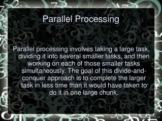
Maximizing Efficiency through Parallel Processing Concepts
Explore parallel processing concepts like algorithms without loops, tree-height reduction, and parallelism in statements for enhanced system performance. Learn about parallel numerical algorithms and techniques. Discover practical applications and systems.

Maximizing Efficiency through Parallel Processing Concepts
E N D
Presentation Transcript
PARALLELPROCESSINGFrom Applications to Systems Gorana Bosic gogaetf@gmail.com Veljko Milutinovic vm@etf.bg.ac.yu
Dan I. Moldovan “Parallel processing from applications to systems” Morgan Kaufmann Publishers, 1993 pp. 67-78, 90-92, 250-260 / 40
PARALLEL NUMERICAL ALGORITHMS • Algorithms Without Loops • Matrix Multiplication • Relaxation / 40
a1 + a2 + a3 + a4 + a5 + a6 + a7 + a8 step1 step2 step3 Algorithms Without Loops • Parallelism Within a Statement An expression is a well-formed string of atoms and operators • an atom is a constant or a variable • operators are arithmetic (+, *, -) or logic (OR, AND) operations / 40
Algorithms Without Loops • Tree-Hight Reduction The tree height of a parallel computation is the number of computing steps it requires The tree hight can be reduced by using • the associativity law • the commutativity law • the distributivity law / 40
((( a + b ) * c ) * d ) ( a + b ) * ( c * d ) step1 step2 step3 Algorithms Without Loops • Tree-Hight Reduction Parallelism provided by associativity / 40
a * ( b + c ) * d a * d * ( b + c) step1 step2 step3 Algorithms Without Loops • Tree-Hight Reduction Parallelism provided by commutativity / 40
a * b * c + a * b ( a * b ) * ( c + 1 ) step1 step2 step3 Algorithms Without Loops • Tree-Hight Reduction Tree-hight reduction provided by factorization / 40
Algorithms Without Loops • Tree-Hight Reduction Tp [E(e)] ≤ [ 4 log ( e -1 )] - 1 E(e) – the expression e – the number of atoms or elements on the right-hand side Tp – the parallel processing time of an arithmetic expression when p processors are used / 40
Algorithms Without Loops • Parallelism Between Statements S1: x = a + bcd S2 : y = ex + f S3 : z = my + x / 40
a b c d e f m step1 step2 step3 step4 step5 step6 step7 bc * * + S1 : x * + S2 : y * + S3 : z Algorithms Without Loops • Parallelism Between Statements / 40
b c d m f e a step1 step2 step3 step4 step5 * * * ea bc mf * * + a+mf mea bcd a+mf+bcd + * bcde a+mf+bcd+mea * + bcdem + a+mf+bcd+mea+bcdem Algorithms Without Loops • Parallelism Between Statements / 40
Matrix Multiplication C = AB cij = aikbkj a( i, j, k ) = aikj b( i, j, k ) = bkji c( i, j, k ) = cijk for i=1 to n for j=1 to n for k=1 to n cijk = cijk-1 + aikbkj end k end j end i for i=1 to n for j=1 to n for k=1 to n a( i, j, k ) = a( i, j-1, k ) b( i, j, k ) = b( i-1, j, k ) c( i, j, k ) = c( i, j, k-1 ) + a( i, j, k ) b( i, j, k ) end k end j end i / 40
Matrix Multiplication Dependece matrix: / 40
Systolic Matrix Multiplication • Processors are arranged in a 2-D grid. • Each processor accumulates one element of the product. • The elements of the matrices to be multiplied are “pumped through” the array. / 40
b1,2 b2,1 b0,2 b1,1 b2,0 b0,1 b1,0 b0,0 a0,2 a0,0 a0,1 a1,1 a1,2 a1,0 a2,0 a2,1 b2,2 columns of b aligment in time b0,2 b1,2 b1,0 b0,0 b2,1 b0,1 b2,2 b2,0 b1,1 a0,0*b0,2 +a0,1*b1,2 +a0,2*b2,2 a0,0*b0,1 +a0,1*b1,1 +a0,2*b2,1 a0,0*b0,0 +a0,1*b1,0 +a0,2*b2,0 a0,0 a0,0 a0,1 a0,1 a0,0 a0,1 a0,2 a0,2 a0,2 rows of a b2,1 b2,2 b0,0 b0,1 b2,0 b1,0 b0,2 b1,1 b1,2 a1,0*b0,1 +a1,1*b1,1 +a1,2*b2,1 a1,0*b0,2 +a1,1*b1,2 +a1,2*b2,2 a1,0*b0,0 +a1,1*b1,0 +a1,2*b2,0 a1,0 a1,1 a1,0 a1,1 a1,0 a1,1 a1,2 a1,2 a1,2 b0,2 b2,0 b1,0 b0,0 b0,1 b2,2 b2,1 b1,2 b1,1 a2,0*b0,0 +a2,1*b1,0 +a2,2*b2,0 a2,0*b0,1 +a2,1*b1,1 +a2,2*b2,1 a2,0*b0,2 +a2,1*b1,2 +a2,2*b2,2 a2,1 a2,0 a2,1 a2,0 a2,1 a2,0 a2,2 a2,2 a2,2 a2,2 / 40
Matrix Multiplication Case 1. The number of used processors: n One processor can be used to compute one column (row) of matrix C. This means that each horizontal (vertical) layer of the three-dimensional cube is done in one processor (loop j is performed in parallel). The parallel time complexity is O(n2) / 40
Matrix Multiplication Case 2. The number of used processors: n2 Each processor may be assigned to compute an element cij of matrix C. In this case both loops i and j are performed in parallel. The parallel time complexity is O(n) / 40
Matrix Multiplication Case 3. The number of used processors: n3 Can the time complexity be reduced to a constant? The lower bound of a matrix multiplication algorithm is O(log n) / 40
Relaxation Updating a variable at a particular point by finding the average of the values of that variable at neighboring points. for i=1 to l for j=1 to m for k=1 to n u( j, k ) = ¼ [u( j+1, k ) + u( j, k+1 ) + u( j-1, k ) + u( j, k-1 )] end k end j end i u( i, j, k ) = ¼ [u( i-1, j+1, k ) + u( i-1, j, k+1 ) + u( i, j-1, k ) + u( i, j, k-1 )] / 40
7 3 4 7 2 5 8 2 3 8 1 4 8 2 4 7 3 4 7 4 3 8 2 3 8 3 2 8 3 3 i=7 7 4 3 7 5 2 8 4 1 8 3 2 8 4 2 i=8 Relaxation k 5 4 3 2 1 j 5 3 2 4 1 / 40
Relaxation Points: (7, 2, 5), (7, 3, 4), (7, 4, 3), (7, 5, 2), (8, 1, 4), (8, 2, 3), (8, 3, 2), (8, 4, 1) belong to the plane whose equation is 2i+j+k=21 The dependence matrix is: / 40
PARALLEL NON-NUMERICAL ALGORITHMS • Transitive Closure G = (V, E) directed graph Is there a connecting path between any two vertices? A = [aij] the adjacency matrix of G aij = 1 if there is an edge (i, j) E and aij = 0 if not A* = [a*ij] the connectivity matrix of G a*ij = 1 if there is a path in G from i to j and a*ij = 0 if not A* is the adjacency matrix for the graph G = (V, E*) in which E* is the transitive closure of the binary relation E A well known algorithm for computing A* is Warshall’s algorithm / 40
PARALLEL NON-NUMERICAL ALGORITHMS • Transitive Closure Algorithm for k=1 to n for i=1 to n for j=1 to n aijk← aijk-1 (aikk-1∩ akjk-1) end j end i end k The dependencies are: / 40
PARALLEL NON-NUMERICAL ALGORITHMS • Transitive Closure Algorithm The dependences are between successive k loops and no dependence lies on the (i, j) planes. All operations on the (i, j) plane can be done in parallel, and the k coordinate becomes the paralllel time coordinate. Thus the total time required isO(n) / 40
j i PARALLEL NON-NUMERICAL ALGORITHMS • Data dependencies for transitive closure algorithm (n=4) / 40
MAPPING OF ALGORITHMS INTO SYSTOLIC ARRAYS • Systolic Array Model • Space Transformations • Design Parameters / 40
Systolic Array Model A systolic array is a tuple (Jn-1, P), where Jn-1Zn-1 is the index set of the array, and PZ(n-1)xr is a matrix of interconnection primitives. The position of each processing cell in the array is described by its cartesian coordinates. The interconnections between cells are described by the different vectors between the coordinates of adjacent cells. The matrix of interconnection primitives is where pj is a column vector indicating a unique direction of a communication link. / 40
Systolic Array Model A square array with eight-neighbour connections j1 00 10 20 01 11 21 02 12 22 j2 J2 = (j1, j2) for 0 ≤ j1≤ 2, 0 ≤ j2≤ 2 / 40
Systolic Array Model A triangular systolic array j1 p1 00 30 10 20 p3 p2 11 21 31 J2 = {(j1, j2) : 0 ≤ j1 ≤ 3, 0 ≤ j2 ≤ 3} 22 32 j2 33 / 40
Space Transformations T is a linear algorithm transformation that transforms an algorithm A into an algorithm Â, defined as: Π: Jn → Ĵ1 S : Jn → Ĵn-1 , space transformation Algorithm dependences D are transformed into SD = P For each dependence di, the product Sdi represents an ((n-1)x1)-column vector. The index point where dependence vector di originates is mapped by transformation S into a cell of the systolic array and the terminal point of the dependence vector is mapped into another processing cell. / 40
Space Transformations Case 1. Given an algorithm with a dependence matrix D and transformation S, find P. Case 2. Given an algorithm with a dependence matrix D and a systolic array with interconnections P, find transformation S that maps the algorithm into the array. / 40
Space Transformations In the second case, the number of interconnections may not coincide with the number of dependences, and equation SD=P cannot be applied directly. The utilization matrixK SD = PK kji = 1, ith dependence utilizes (or is mapped into) communication channel j kji = 1, ith dependence does not map into channel j Numbers larger than 1 may be possible (0 ≤kji), and indicate repetitive use of an interconnection by a dependence A dependence may map into several interconnections. The number of time units spent by a dependence along its corresponding connections cannot exceed the time alocated by the transformation to that dependence. ( 1 ≤ Σjkji≤ Πdi ) / 40
Space Transformations Example: for j0=1 to n for j1=1 to n for j2=1 to n S1: a(j0, j1, j2 ) = a (j0, j1+1, j2 ) * b (j0, j1, j2+1 ) S2: b (j0, j1, j2 ) = b (j0, j1-1, j2+2 ) + b (j0, j1-3, j2+2 ) end k end j end i / 40
Design Parameters ĵ = (ĵ0, ĵ1, ĵ2) Ĵ ĵ = Tj The first coordinate ĵ0 indicates the time at which the computation indexed by the corresponding j is computed. The pair (ĵ1, ĵ2) indicates the processor at which that computation is performed. At what time and in what processor a computation indexed by (3, 4, 1) is performed? The transformed coordinates are (ĵ0, ĵ1, ĵ2)t = T (3, 4, 1)t = (2, 8, 3)t , meanig that the computation time is 2 and the processor cell is (8, 3). / 40
Design Parameters The first row of the transformed dependences is: Each element indicates the number of time units allowed for its respective variable to travel from the processor in which it is generated to the processor in which it is used. Only two interconnection primitives are required: (0, 1)t and (1, 0)t / 40
Design Parameters Systolic array: / 40
Design Parameters Cell structure: b a b Delay 1 time unit Delay 2 time units Delay 1 time unit * + b a b / 40