Download
1 / 53
530 likes | 550 Views
Dive into advanced data structures like Quad trees, k-d trees, TV trees, R trees, and their applications in range queries and k-nearest neighbor searches. Explore complexity, similarity functions, and potential applications across domains like image databases, medical databases, DNA databases, time series, military surveillance, and network models. Discover the seven-layer OSI network model and networking techniques.

E N D
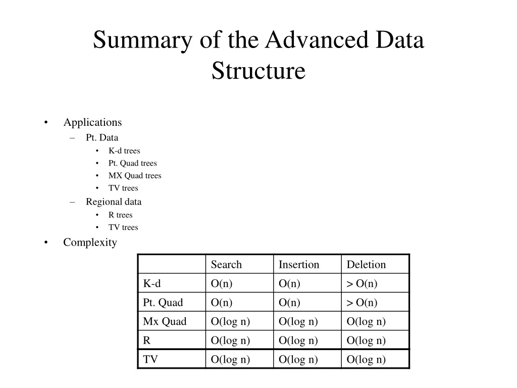
Summary of the Advanced Data Structure • Applications • Pt. Data • K-d trees • Pt. Quad trees • MX Quad trees • TV trees • Regional data • R trees • TV trees • Complexity
Two Important Queries • Range query • Given a range specified in the query, expect to return all the data points or regions that are within the query range • Recursively branch down all the children • Cut branches that do not intersect with the query range • k nearest neighbor search • Given a spatial point or a spatial region in the query, expect to return the sorted top k data points or spatial regions in the database that are closest to the query point or query range • Need to define carefully the “similarity” function • Points: Euclidean distance • Regions: • If ignore the “shape” information, Euclidean distance may be fine • If ignore the “distance” information, a pure shape similarity function may be defined • When both need to be taken care, some sort of combination is expected • Essentially all the search engines employ k nearest neighbor search to return a retrieval • Same idea of recursive branching down • Same idea of search by exclusion
k Nearest Neighbor Search • Search from the root arbitrarily (say breadth first or depth first) to obtain k different distances (may have to visit more than k nodes) • Sort the k distances in an array upper bound for the kth nearest distance • Start from the root to initiate the search • If the “distance” from the query to the boundary of the region of the node is larger than the upper bound, cut the subtree • Else, compute the “distance” from the query to the node • If the “distance” smaller than the upper bound, update the k distances in the array (also updated the upper bound) • Recursively search the children • The k “distances are updated along with the search, and are made closer and closer to the actual k “disntaces” • The “distance” may be actually Euclidean distance for points, or active distance for points or regions in TV trees, or any defined similarity incorporating shape and distance • The same algorithm may be applied for all the advanced data structures
Potential Applications • Image databases • Image features may be in high dimensional space (e.g., using histogram as feature) • Medical databases • 1D objects (e.g., ECG), 2D images (e.g., X-ray), 3D images (e.g., MRI), after indexing they may all end up with features in high dimensional space • Time series • Such as financial database, features used such as DCT/DFT in high dimensional space • DNA databases • All the strings are sequences of letters in an alphabet; if we have m letters in total, and use n-gram features, we are talking about a dimensionality of m^n in the feature space • Substring matching • For example, automatic spelling correction in which you have partial information correct but you have a whole dictionary of correct information; how to search the whole dictionary? • Also you have a partially correct address/name in postal service, and would like to intelligently “guess” the correct complete delivery address • In all cases, the dimensionality of the feature space is exponentially large • Military surveillance • Bombing areas determination • Deployment planning
Network Model Compilers • The onion structure of OS • The same layer idea drove ISO to design the 7-layer OSI network model: • Layer-7 Application: provides a communications service interface to an application • Layer-6 Presentation: looks after the presentation aspects of the data; if the nodes on the two ends of the link use different codes for data representation, it is the responsibility of this layer to perform code conversion • Layer-5 Session: responsible for establishing and terminating a session of activity between two nodes • Layer-4 Transport: responsible for accepting messages from the upper layers and breaking these into packets suitable for the lower layer protocols; also responsible for monitoring the quality of the link and for selecting one path if many alternative paths are available • Layer-3 Network: performs the task of routing the data in a multinode network • Layer-2 Data Link: makes sure that data are transmitted reliably even over unreliable media • Layer-1 Physical: responsible for actually transmitting and receiving the stream of bits that comprise data as well as control information OS Networks Applications
Networking Techniques • Any physical network may be modeled as a star-like generic topology to provide PTP (point to point) communications between any two nodes in the network • Two basic techniques to implement this generic structure • Switch sharing: all nodes are connected to a switch via PTP links. This switch may be in turn a collection of other switches and links. Any data exchange between nodes is carried out by the switch. • Media sharing: all nodes are connected to a single shared media. This shared media must be used for all data exchange operations 2 3 1 4 Network 8 5 7 6
Media Sharing • Also called multiplexing • Trunk line: the high-bandwidth line connecting two end devices • Four different implementations • Frequency Division Multiplexing (FDM): divides the trunk bandwidth into many smaller bandwidth channels and carries signals in these channels simultaneously through the trunk line • Need to pay attention to leave gaps between two neighboring sub-bandwidths (called guard bands) to avoid cross talk • Time Division Multiplexing (TDM): divides time into distinct time-slots and shares these time-slots between different branch ports • Two implementations • Bit interleaving: each time-slot is allocated to one bit from one branch port at each time • Character interleaving: each time-slot is allocated to one character from one branch port at each time • Pure TDM: the time-slots are allocated in a fixed cyclic order between all the branch ports • Disadvantage: any time-slot not used by a branch port is wasted • Statistical Time Division Multiplexing (STDM): allocates time-slots to branch ports based on statistical data on the utilizations of different branch ports --- more time-slots to busy ports • Improve the utilization of the trunk line • Order of time-slot allocation is not fixed each data unit transmitted in a time-slot must carry the address of the originating branch port to be able to be picked up by the matching port at the other end • Contention Based Media Sharing (CBMS): trunk line is shared by all the branch ports in the way that at any time, only one signal can exist in the trunk line at any time, only one port can transmit data (speak), and all other ports can only receive the data (listen)
Switch Sharing • Network cloud consists of a collection of switching nodes connected by PTP links • The switching nodes try to move data from node to node; every node is connected to the network via a switching node • Two main implementations: • Circuit switching: dedicated end-to-end circuit is established between the two communicating nodes by using physical connections in the switching nodes; the links between the various user nodes and switching nodes are fixed while the connections within the switching nodes are dynamic and need to be switched to establish the required end-to-end circuit; 3 phases: • Establish a circuit • Transfer information • Disconnect the circuit • Packet switching: data files are broken down into packets before transmission; each packet comprises a packet header and a fixed or variable length data section, followed by a CRC (cyclic redundancy check) for error detection • Avoid retransmission of the entire file in case of any error • Each packet is treated as a separate entity for the entire duration of its transmission from one user node to another • Two ports connected by a logical link can pass packets to each other via buffers, even in the absence of a direct electrical connection • On a circuit switching node, one port can be connected to only one other port at a time, while on a packet switching node, many logical connections can exist from one port to other ports • Two main approaches: • Datagram • Virtual circuit
Packet Switching • Datagram: Each packet is given a sequence number, and treated as an independent entity • No end-to-end dedicated connection is established between two user nodes • Packets may route through different paths, and may arrive in destination in different orders • A final assembly is required at the destination to put back packets into the original file • Virtual circuit: combines the datagram idea with the circuit switching technique • An end-to-end path is selected and a virtual circuit is established before any data packets are transmitted • No end-to-end physical connection is actually established --- data packets are passed from one port to the other via buffers, and packets may have to wait in queues in transmission • No need to attach the destination address to each packet, though each packet must include a virtual circuit identifier • Three phases: • Virtual circuit establishment • Information transfer • Circuit disconnection • Two variations of the original packet switching technique • Frame relay: • packets are called frames --- variable length packets • reduced error checking • Cell relay: also called Asynchronous Transfer Mode (ATM) • Packets are called cells --- fixed length data packet • Transmission is made through virtual channels • No need to append destination address to each cell
ATM Cells • Cell size • Variable packet size has nice characteristics dynamically saves storage and transmission space for small data chunks; dynamically minimizes the transmitted packets based on the maximum cell sizes • ATM cell size is fixed at 53 bytes (5 bytes header + 48 bytes payload data) easy implementation (especially hardware implementation); short transmission latency • Cell format • Depends on two scenarios • User-Network Interface (UNI) • Network-Network Interface (NNI) • Format Field Name Number of bits -------------- ------------------ Generic Flow Control (GFC) 4 (UNI) or 0 (NNI) Virtual Path Identifier (VPI) 8 (UNI) or 12 (NNI) Virtual Channel Identifier (VCI) 16 Payload Type (PT) 3 Cell Loss Priority (CLP) 1 Header Error Control (HEC) 8 Payload Data 384
ATM Cell Format • Generic Flow Control (GFC): does not appear in the cell header in the internal network; only used to control the cell flow at the local user-network interface; not used at present • Virtual Path Identifier (VPI): “global” path identifier when communications are only required between two switches through “global” network (e.g., internet) • Virtual Connection Identifier (VCI): “local” path identifier when communications are also required through “local” network (e.g., within an organization’s intranet) • Payload Type (PT): 1st bit = 0 user data; = 1 network management/maintenance PT Coding Interpretation ------------- ---------------- 000 User data cell, congestion not experienced, SDU (Service Data Unit) type = 0 001 User data cell, congestion not experienced, SDU type = 1 010 User data cell, congestion experienced, SDU type = 0 011 User data cell, congestion experienced, SDU type = 1 100 OAM (Operations, Administration, and Maintenance) segment associated cell • OAM end-to-end associated cell 110 Resource management cell 111 Reserved for future function • Cell Loss Priority (CLP): used for guidance to control network congestion; 0 higher priority and should not be discarded unless no other alternatives; 1 else • Header Error Control (HEC): determines whether there are errors in the header based on the 8 bit data and the remaining 32 bits in the header; if just one bit error, may be able to correct it; otherwise, just detect and determine whether there are errors
ATM Service Categories • Real time service: high demands on network delay and jitter control • Constant bit rate (CBR): commonly used for uncompressed audio and video information; Examples: • Videoconferencing, interactive audio (e.g., telephony) • Audio/video distribution (e.g., television, distance learning, pay-per-view) • Audio/video retrieval (e.g., video-on-demand, audio library) • Real time variable bit rate (rt-VBR): intended for time-sensitive applications, i.e., requiring tightly constrained delay and delay variation; typically for bursty sources; Example: • Video service to several clients in parallel with transmission of compressed video data Given the network bandwidth, distribute the video burstiness into different clients to maximize the bandwidth usage flexibility • Non-real-time services: for applications that have bursty traffic characteristics and do not have tight constraints on delay and delay variation greater flexibility in network and greater usage of statistical multiplexing to increase network efficiency • Non-real-time variable bit rate (nrt-VBR): for applications with expected traffic flow characteristics; need to specify information like peak cell rate, average cell rate, and a measure of how bursty the cells may be network can allocate resources to provide relatively low delay and minimal cell loss; Example: • Airline reservations, banking transactions, processing monitoring • Unspecified bit rate (UBR): For applications that can tolerate variable delays and some cell losses; typically used for the “left-over” network capacity for these applications after servicing higher demand applications; service based on UBR is called best effort service; Example: • Text/data/image transfer, messaging, distribution, retrieval • Remote terminal (e.g., telecommuting) • Available bit rate (ABR): like nrt-VBR, certain network characteristics need to be specified; unlike nrt-VBR, only the peak cell rate (PCR) and min. cell rate (MCR) need to be specified s.t. at least MCR will be assured while higher bit rate will be serviced as much as possible; ABR and UBR typically share the left over network bandwidth after CBR and VBR services; service based on ABR – closed loop control;Example: • LAN interconnection
ATM Bit Rate Services 100% ABR and UBR Percentage Of Network Capacity VBR CBR 0 Time
ATM Adaptation Layers • Use of ATM needs an adaptation layer to support information transfer protocols not based on ATM motivation to define ATM Adaptation Layers (AAL) • Services provided by AALs • Handling of transmission errors • Segmentation and reassembly, to enable larger blocks of data to be carried in the information field of ATM cells • Handling of lost and misinserted cell conditions • Flow control and timing control • AAL protocols | Class A | Class B | Class C | Class D Timing relationship | | | B/w source and destination | Required | Not required Bit rate | Constant | Variable Connection mode | Connection Oriented | Connectionless AAL Protocol | Type 1 | Type 2 | Type ¾ | | Type 5 |
Integrated Services Digital Network • ISDN was designed to provide data rates in the range of Kbps to Mbps • Higher data rates (Mbps to Gbps) capability over ATM was called broadband-ISDN • The principle underpinning the development of the ISDN was to provide an end-to-end digital network that can integrate all types of services which may include voice, digital data, text, and video • ISDN also provides bandwidth on demand • User is expected to use only as much bandwidth as required for the application at hand • User pays only for the time for which the service is available • Synchronous Optical Network (SONET): data transmission service based on optical transmission; a transport service that can be used for advanced network services such as broadband ISDN (B-ISDN), Fiber Distributed Data Interface (FDDI), and High Definition Television; uses optical fiber as media provides much higher bandwidth • SONET is used in conjunction with the ATM for the B-ISDN; SONET’s Optical Carrier (OC) standards: OC level Transmission speed OC-1 51.84 Mbps OC-3 155.52 Mbps OC-12 933.12 Mbps OC-24 1.244 Gbps OC-48 2.488 Gbps
ISDN Channels • A-Channel: analog channel included to make ISDN connections upward-compatible with the current analog telephone lines • B-Channel: also called bearer channel; expected to “bear” or carry high volume traffic such as digitized voice, video, and other data; single B-channel only provides a 64 Kbps bandwidth; for high volume traffic, typically a number of B-channels are required • C-Channel: low speed digital data transfer; designed to work with older-style dumb terminals requiring a bandwidth of less than 16 Kbps • D-Channel: also called data channel; used for out-of-band signaling • Out-of-band signaling: the control signals are not mixed with the data stream, but are carried on a separate circuit allows the channel carrying user data to be used more efficiently • Examples of the out-of-band signals include on-hook and off-hook signals • Also called common channel signaling • Summary: Channel Designation Channel Type Bandwidth Application Area A Analog 3 – 4 KHz Analog voice B Digital 64 Kbps Digitized voice/data C Digital <= 16 Kbps Low-speed data D Digital 16 or 64 Kbps Signaling or data
ISDN Interfaces • ISDN services are provided to users as ISDN interfaces • Each ISDN interface comprises a few ISDN channels • Typical ISDN interfaces • Basic Rate Interface (BRI): targeted to provide a simple interface to a desktop; includes a phone connection and a digital interface for the desktop computer; D-channel is used for signaling and the two B-channels provide a bandwidth of 128 Kbps for data transmission • Primary Rate Interface (PRI): 23 to 30 B channels are combined to provide a bandwidth of 1.544 to 2.048 Mbps; a D-channel is used for out-of-band signaling; used for video conferencing apart from other multimedia applications • Hybrid Interface (HI): allows connections that use a hybrid of analog and digital communication • For high-end multimedia networking, B-ISDN system need to be developed • Summary: Interface Name Channels Included Combined Bandwidth Application Area BRI 2B+D 144 – 192 Kbps Digitized voice/data interface PRI 23B+D 1.544 Mbps High-volume data, data, 30B+D 2.048 Mbps LAN to LAN connection HI A+C Analog voice + 16 Kbps For a hybrid connection for transition
Classification of Temporal Relationships Based on Three Aspects • Object Stream Interactions • Intramedia: temporal relationship between objects of one stream • Example: Animation without sound • Intermedia: temporal relationship between objects of two parallel streams • Example: Video clip with sound • User interaction: temporal constraints in terms of response time • Example: Education/entertainment system • Media Levity • Live: presentations with info captured, transmitted, and presented in real time • Example: Video conference • Stored: presentations with info captured and stored in secondary storage systems • Example: Video-on-demand • Mixed: combination of live and stored presentations • Example: Collaborative conference • Media Synchronization • Asynchronous: no well-defined time relationship between objects from one or more streams • Example: Text entry on a keyboard • Synchronous: well-defined time relationship between objects from different streams • Example: Video with sound • Isochronous: well-defined time relationship between objects from the same stream • Example: Sound
Specification of Temporal Relationships • Relative time specification • Seven basic Relative Temporal Relationships (RTR) [Are they independent? Given two temporal events A and B, how many different possible combined events?] • A before B • A meets B • A during B • A overlaps B • A starts B • A ends B • A equals B • Temporal transformations • Inverting • Scaling • Shifting • Absolute time specification • Instant Based Specification: specifies the beginning and ending times • Interval Based Specification: specifies the beginning time and the duration • Inexact Timing Specification: gives a lower bound and an upper bound for a duration over which an object may be played back • Example: a music starts soon after an image displayed, and as soon as finishes, the image fades out
Synchronization Accuracy Specification • For isochronous and synchronous systems, the level of synchronization is specified and thus controlled by a set of parameters --- SAS parameters • Delay: end-to-end transmission/processing/presentation time --- total delay called latency • In an interactive application, delay is the response time • In a stream application, delay is the total time taken by an object to go from source to destination • Jitter: the instantaneous difference between the desired presentation times and the actual presentation times of steamed multimedia objects • Intramedia jitter: instantaneous asynchrony in isochronous object streams • Intermedia jitter: instantaneous asynchrony in objects from two streams • Skew: the average difference between the desired presentation rate and the actual presentation rate of streamed multimedia objects • Intramedia skew: asynchrony between stream objects and the reference clock • Intermedia skew: asynchrony between objects from two or more streams and the reference clock • Error rate: measurement of how much error occurred • Bit Error Rate (BER) = Bits in error / Total number of bits transmitted • Packet Error Rate (PER) = Packets in error / Total packets transmitted • Classic data transmission protocols require retransmission in case packets are in error • In multimedia applications, retransmission may not always be the best option
More Network Parameters • SAS parameters only specify the need of an application expected • The actual performance of a network is characterized by Network Performance Parameters (NPPs) • Throughput • The bit rate of a network only specifies the maximum transmission rate • The actually bit rate varies over time, and typically is below the maximum rate due to collision, protocol overhead, network congestion, etc. • The average performance (net bandwidth) is called throughput = #bits transferred/time taken • In terms of different types of applications, two scenarios of bit rates • Constant bit rate (CBR): certain applications have constant bit rates, e.g., uncompressed audio or video transmission • Variable bit rate (VBR): certain applications have variable bit rates, e.g., compressed audio or video signals • In case of VBR, the variation in the traffic is defined as burstiness, and is specified as Peak Bit Rate (PBR) and Mean Bit Rate (MBR); then Burstiness ratio = MBR/PBR • Delay Variance • Refers to the fact that different packets experience different delays in the network • Also called delay jitter • While delay only wastes time in waiting for the response, the delay jitter leads to unacceptable presentation quality; this parameter is set in terms of an upper bound; e.g., for TV quality video, delay jitter < 10ms; for high fidelity stereo music, or compressed video, the delay jitter < 1ms
Quality of Service (QoS) • Users require different quality presentations at different times • Different quality presentations map into different parameters different requirements for the network performance • QoS is a subjective matter, and also incorporates a set of parameter ranges as opposed to a set of precise parameters three different perspectives • User perspective: a function of the ability of human sense to distinguish between different quality presentations. • Parameters include image size, color bits, voice quality (sampling rate and sample size), steadiness of the picture (jitter and skew), as well as the cost expected to achieve the quality specified • Application perspective: a description of the application performance • Parameters mainly include all SAS parameters: delay, jitter, skew, and error rate; for an interactive application (e.g., virtual reality systems), also include response time • Transmission perspective: a description of the transmission performance • Parameters mainly include all NPP parameters: throughput, burstiness, and delay variance
QoS Venn Diagram Application Perspective (SAS Factors) Delay, Jitter, Skew, Error Rate User Perspective Image Size, Color Bits, Voice Quality, Steady Picture, Cost Response Time Delay Jitter Throughput, Burstiness, Compression, Transport Technique Transmission Cost Transmission Perspective (NPPs)
QoS Guarantees: Definitions and Challenges • Two ways for guaranteeing QoS: • Deterministic: set up a bound on performance of all packets within a session • With real time traffic, no cells would be delayed > D time units on an end-to-end basis • No cell loss occurs • Statistical: set up no more than a specified fraction of cells below a certain specified value • With real time communication, no more than x% of the cells would experience a delay > D • With cell loss, no more than x% of the cells in the session are lost • Challenges of characterizing QoS: • Multimedia traffic exhibits correlated, time-varying behavior that is significantly more complex than that of traditional data network traffic • In multimedia communications, QoS requirements are defined in an individual, per-session basis; no longer sufficient to simply determine the performance of the aggregated network traffic performance must be characterized at the finer-grained, per-session basis • Performance must be evaluated in a multi-hop network setting, in order to accommodate the complex interactions among sessions intra-session and inter-session packet interactions must be considered in this evaluation • Four basic approaches to ensuring QoS (J. Kurose) • Tightly controlled approach • Approximate approach • Bounding approach • Observation-based approach
Tightly Controlled Approaches • Make sure a non-work multiplexing (queuing) discipline such that an individual session’s output traffic characteristics (i.e., after being multiplexed with other sessions at a switch output port) are the same as that session’s input traffic characteristics (i.e., before multiplexing) • Classic example: stop and go • Define time frames • Make sure that a cell arriving in one frame at a switch’s input is never transmitted over an output link during the same time frame in which it arrived • A cell may have to be held in the switch’s output buffers while the output link is purposefully allowed to go idle • Pros and cons: • Pros: simple characteristics of the session’s performance (e.g., deterministic evaluation) • Cons: • A fairly sophisticated, non-work-conserving queuing discipline must be implemented which tracks each individual session’s timing requirements on a per-session basis • A session admitted into the network essentially “reserves” bandwidth based on its peak rate --- effectively resulting in a form of circuit-switching classes of traffic with high peak-to-average traffic rates only utilize the links for a small fraction of their “reserved” amount of time, potentially leaving the links significantly underutilized
Approximate Approaches • Traffic sources at the network’s edge (and also within the network) are characterized by relatively “simple” models; in order to determine whether or not the multiplexed sources will receive their required QoS, the queuing behavior of the multiplexed traffic streams is then analyzed based on this “simple” model as well as the pre-defined measure of interest (e.g., packet loss, maximum delay, etc.) • Example: on/off simple model for traffic source: alternate between on-period (during which cells are typically generated periodically) and off-period (during which no cells are generated) • Pros and cons • Pros: • “simple” admission control cheap computation in admission control well-suited for real-time, online implementation • Due to this “simple” admission control, many simple scheduling policies may be applied (e.g., FCFS) • Able to take advantage of statistical multiplexing gains, potentially carrying traffic with peak rate exceeding link capacity (while tightly controlled approaches can’t) • Cons: • “approximate” not clear about the extent to which more complicated sources can be characterized by the relatively simple approximate models • View all the traffics within a network the same as (approximated by) the edge traffic model not true in real situations especially when the network has very “deep” nodes • Parameters determined at the edges are local while parameters of QoS are expected for global performance may not be matching together
Bounding Approaches • Characterize the QoS of the whole network in terms of one of the following bounds for each node: • Deterministic bounds • Statistical bounds • Example: Packetized Generalized Processor Sharing (PGPS) • Pros and cons: • Pros: • More accurately and realistically reflects the actual performance for each multiplexed node (as compared with, say, the approximate approaches) • Able to model each node within a network • Cons: • Reliance on the ability to bound the maximum length of each queue’s busy period for a given set of traffic specifications if this condition is not satisfied, no bound can be computed
Observation Based Approaches • Previously made measurements of certain types of traffic sources are used to characterize the current traffic model, and to determine the traffic acceptance decision • Example: bandwidth requirements of already admitted, token bucket-controlled, sessions are determined from the current, measured behavior of these sessions rather than the traffic parameters declared by these traffics when they first arrived to the network; this measured behavior, together with the declared parameters of an arriving traffic, are then used in making the traffic acceptance/rejection decision for the incoming traffic • Note that in this example, no firm QoS guarantees can be made since traffic admission (and thus QoS “guarantee”) is based on measured traffic loads at traffic admission time --- loads which may change once the traffic is admitted traffic receiving guarantees based on observation are referred to as receiving “predictive service” • Pros and cons • Pros: • Traffic parameters for each session are not required, but each traffic session must be one of a pre-defined set of classes and its traffic presumably corresponds to the traffic characteristics of that class if the guarantees are to be reliable • Network may be more fully utilized based on the predictive service rather than guaranteed service • Cons: • Open issues including the effects of different measurement/estimation techniques on the protocol, the overhead involved in measurement, the influence of the number of multiplexed sessions on the reliability of the guarantees, and a thorough study of the mechanism in a larger network environment
Audio Transmission Control • Background: • Audio/video transmission: network congestion frame losses • Two approaches • Resend --- not realistic for audio/video transmission • Recovery at the receiver side --- approach under consideration • Advantage: in audio/video transmission, certain frame loss is not critically noticeable • ATM packet approach (J-C. Bolot and A. Fega-Garcia) • Focus on rate and error control mechanisms • Packet structure: audio packets are sent from the source to the destination(s) using IP, UDP, and RTP; each audio packet is associated with a timestamp measuring end-to-end delays, and a sequence number used to detect packet losses • Loss analysis: • ln: boolean variable --- 1 for packet n being lost and 0 otherwise • ulp = E[ln] --- average loss --- does not address the correlation between successive packet loss • clp = P[l_(n+1) = 1|ln = 1] --- conditional probability to address the correlation • Using PCM coder with 320 byte packets (40 ms of speech) between INRIA Sophia Antipolis and University College London (UCL) ulp = 0.21 heavy congestion • Number of consecutive losses is mainly focused on the range < 8
Packet Loss Recovery • Recovery is necessary when the number of lost audio packets is higher than tolerated • Two general approaches: • Automatic Repeat Request (ARQ) --- closed loop control mechanism --- packets not received at the destination are retransmitted; not good for live audio applications because • Increase end to end latency • Do not scale well to large multicast environments • Forward Error Correction (FEC) --- open loop control mechanism --- redundant information is transmitted along with the original information s.t. (at least some of) the lost original information may be recovered; good for live audio applications • Provide reliability and quality without increasing latency • Effectiveness of FEC depends on the characteristics of the packet loss process in the network only effective if lost packets are dispersed throughout the stream • Conventional FEC approach: after sending every n packets, a redundant packet is sent based on the exclusive-OR of the n packets • Pros: able to recover single loss; simple to implement • Cons: increases the send rate at the source by 1/n; adds latency as n packets need to be received before recovery done • New approach of FEC: for each packet i, in addition to the original PCM data, add a redundant version of packet i-1 with a low bit rate coder (such as LPC or GSM) • Pros: • Recover isolated losses with much lower latency (only need to wait for one packet for recovery) • Little overhead for each packet (e.g., with LPC coding, 24 bytes added for every 320 bytes packet) • Capability to extend to recover multiple consecutive losses (e.g., add LPC or GSM versions of packets i-1, i-2, etc. in packet i) with the cost of adding more overhead in each packet • Cons • The receiver needs to have the capability of decoding mixture of PCM and LPC or GSM stream
Media Synchronizations • Motivation: synchronizations are required for continuous types of media • Classifications: • Synchronizations between streams of the same media types • Example: stereo audio files • Synchronizations between streams of different media types • Example: video stream with audio streams, power point presentation file with audio sounds • Essentially execution of a retrieval plan • Basic approach: packetization of the streams to make sure the corresponding frames (cells) are played at the scheduled times • Examples • IMB Bamba • OGIST Distributed real-time MPEG video audio player • UIUC Vosaic project
Design of Server & Client Communications with Synchronized Streams • Whole system has two parts: server and clients • Clients may be multiple clients • Broadcast model • Server responsible for listening to the request from clients, and launches threads to serve clients • Client sends request to server • If request approved, client starts threads to receive data, and sends a start message to server to start displaying video session • Upon receiving the start message from the client, server begins to read data from disk files and sends them to the client through network • Two streams are synchronized through buffers • Packets from the two streams are assembled together to playback at the client side
Server Video Sending Thread AdmittedClientSet AdmittedClient Network Audio Sending Thread Feedback Thread Disk Read Thread
Server, Cont’d • A dialog based MFC application, written in Visual C++ 6.0 under Windows 2000 • CStreamVideoServerApp is the class of application, which has a data member named StreamVideoClientSet, a pointer to the AdmittedClientSet class • AdmittedClientSet keeps track of all the admitted clients • Each AdmittedClient has a video data buffer, and an audio data buffer with three threads • Video sending thread --- sending out video packets; increments seq. number for each packet • Audio sending thread --- sending out audio packets; increments seq. number for each packet • Feedback thread --- gets feedback messages from client • DiskReadThread serves all clients • Always browses over AdmittedClientSet • Read data from disk files • Write data to buffers of each AdmittedClient (readaudio() and readvideo()) • If a buffer is full, DiskReadThread does not wait, and skip the buffer moving to the next one • Feedback messages are used to synchronize the transmission between server and client • At the beginning, CListenAdSocket is started to listen to requests; when a request is received, creates a CServerAdSocket to serve the client; CServerAdSocket reads the request from the client and processes it; if the request is approved, it adds a new AdmittedClient to the AdmittedClientSet and starts the three threads in the AdmittedClient; meanwhile, DiskReadThread is started to serve all the AdmittedClient.
Client Request Admission MultiMediaRealTimeStream File Video/Audio Assembly Thread Video Receiving Thread Client Buffers (4) File Audio Receiving Thread Feedback Thread
Client, Cont’d • Each client has MultiMediaRealTimeStream object, responsible for getting video from server and sending feedback messages back to server, as well as assembling the file (for simulation of playing back the synchronized audio/video) • When opened, asks for admission; if approved, start four threads: • Video receiving thread (receive video packets from the server) • Audio receiving thread (receive audio packets from the server) • Audio/Video assembly thread (assemble audio/video data into files) • Feedback thread (synchronize server sending and client receiving data) • Four FlowControlBuffers • Audio seq. number • Audio packets • Video seq. number • Video packets • MultiMediaRealStream keeps reading data from the buffers at a constant rate (to simulate the playback) • Audio/video assembly thread takes the data into an audio file and a video file
Buffer Management Writable items Read pointer Write pointer Readable items
Synchronization b/w Server & Client • Server starts to send data every Interval time • Client receives data and puts them into the client buffers • The client buffer has a threshold H • If the data in the buffer is less than H percent, the client sends a FASTER message to server • After server gets FASTER, decreases Interval • Client keeps sending FASTER to server till the client buffer reaches H • Client sends SLOWER message to server • Server increases Interval after receiving SLOWER • Finally the client buffer is kept around H
Synchronization b/w Audio & Video • Server and client need to work together to synchronize the transmission • Server: • Before sending out each audio or video packet, adds a sequence number on it • Sequence number is an order number of the packet • Packet size is fixed • Video packet one frame at the rate of 25 frames/second • Audio packet 1/25 of one second samples • Client: • Four FlowControlBuffers for audio seq. number and data, and video seq. number and data • When client receives a packet (audio or video), writes it into the corresponding data buffer, then writes the seq. number into the corresponding seq. number buffer • AssemblingThread reads the audio data first • If there are no audio data network is congested • If there is an audio packet, check the video data buffer • If there is not video data, keeps reading and assembling audio data • If there is a video data packet, check the sequence number of the video packet with that of the audio packet • If the video packet seq. number < the audio packet seq. number, skip (drop this video packet and read the next video packet till the video packet seq. number equals the current audio packet seq. number
IBM Bamba • http://www.AlphaWorks.ibm.com (1998) • Used on the official 1996 Olympics Web site to distribute audio and video clips of the games • 100,000 users installed the Bamba plug-ins and played clips from the “Sights and Sounds” pages of the Web site • Clips were offered at two target bit rates: 24 Kb/s for modem-connection users and 100 Kb/s for ISDN and LAN-connection users • Old --- now migrated to HotMedia http://www-4.ibm.com/software/net.media/ • Goals: • Stream audio and video across the Web through very low bit rate connections • Audio is sufficiently compressed to stream over modem connections at 14.4 Kb/s • Video is compressed at 28.8 Kb/s • Allowed to adapt to higher bit rate automatically • When streaming is not possible due to network congestion or insufficient bandwidth, the receiving client automatically calculates how much data to preload in order to maintain continuous playback • Distinctive features of Bamba: • Designed to run over the currently existing network infrastructures --- able to deal with heterogeneous nature of the network and the unpredictable congestion behavior of the traffic • Both the audio and video compressions are based on standard algorithms and can be performed by standards-compliant decoders • Uses either a standard HTTP server or an enhanced video server running RTP over UDP/IP • Implemented either as a helper application which runs outside a Web browser, or as a browserplug-in which enables application developers to embed audio and video clips easily within an HTML document, or as a Java applet which can be downloaded directly from a Web server containing Bamba clips without requiring special software installation at the client
Bamba Technologies • Streaming architecture • Server: standard HTTP web server which contains the stored Bamba audio and video files; Bamba files may be created through standard HTML pages, and then loaded onto and accessed from a standard HTTP server • Client: web browser and bamba audio and video plug-in software; plug-ins are standard Netscape-defined plug-in API • Since the underlying transport protocol used by HTTP is TCP/IP, no special provisions are required for handling packet loss within the network Bamba audio/video files are treated like any other HTTP objects; if selected, a Bamba clip is transferred to a client as fast as TCP/IP can move it, and the client begins decoding and displaying the Bamba file as soon as the first few bytes arrive additional advantage: Bamba streams can traverse firewalls with no special configuration requirements due to using TCP/IP as the underlying protocol • Audio/Video technology • Audio uses G.723 standard with fixed sampling rates. • Video uses H.263 compression standard (successor of H.261) --- uses DCT and frame structure similar to MPEG • Difference: MPEG uses I and P frames while H.263 uses I and P blocks (8 x 8 pixels) reduces size variance between frames and adds flexibility in selecting the refresh distance between I-blocks for different regions of the video image • H.263 can deliver video over very low-bit-rate (<64Kb/s) dedicated connections; in low bit rate range, H.263 outperforms H.261 by a 2.5:1 ratio of signal-to-noise ratio improvement • YVU color model with CIF, QCIF, SQCIF, 4CIF, and 16CIF formats
Bamba Technology • Dynamically adjusted frame rate control algorithm automatically in place fully take advantage of the trade-off balance between frame rate and image quality while still maintaining constant bit rate • Larger frames are dedicated to scene changes or motion-intensive scene, followed by significant frame drop or even no data at all after that • Keep the net transmission rate close to a constant • Frame structure --- synchronizations between audio and video streams • Audio and video are interleaved into a single file to simplify the server function; the server treats a Bamba file as the same as any other data file; audio and video data are interleaved proportionately to maintain a synchronous playback of both streams at the client • Bamba frames consist of a 240 byte segment of audio and a 240 b/a byte segment of video, where a and b are the audio and video rate, respectively • Streaming control --- synchronizations within the stream • Reality: network characteristics are very unpredictable and typically based on a “best-effort” environment no guarantee that resources are available to play a clip smoothly • Has a built-in rate monitor that dynamically evaluates the effective data-transfer rate (c) of a selected audio or video clip and compares this to the specified bit rate (a + b) for the clip, which is contained in the clip header • If a + b c, the clip may be played immediately • Else, a fraction of the clip is buffered sufficiently for the clip to play smoothly once playback is started; the amount of prebuffering is d = L (1 – c/(a+b)), where L is the clip length; this calculation is performed on the basis of the initial download rate and again any time the buffer underflows
Bamba’s Error Handling • Due to frame loss, more I blocks encoded, more reliable • I-block encoding exploits only the spatial redundancy within the block in the compression process, while P-block encoding exploits both the temporal and spatial redundancies of the video; more P blocks encoded, more serious error propagation propagation stops when all corrupted regions are updated by I-blocks • On the Internet, since UDP/IP packet contains several frames, once a packet is lost, all the frames are lost also and cannot be recovered errors begin to propagate • For non-live applications, knowledge about the interdependence among blocks in a sequence can be obtained from the dependencies reflected by the motion vectors it is possible to assign a measure of importance to a pixel or a block by counting the number of pixels or blocks that depend on it; this operation is anticausal, i.e., traversing backward in time; the higher the dependence on a block, the more critical it is that this block be correct and that it be encoded as an I-block dependence chains may be broken by encoding intermediate blocks in the chain as I-blocks • Note that this counting is accumulative (e.g., if block A in frame 3 depends on block B in frame 2, and block B in frame 2 depends on block C in frame 1, then the number of counts of dependence in frame 1 is 2) form a dependence tree for a sequence
Bamba’s Error Handling • Algorithm of selecting a target I-block count, M, for the number of I-blocks to be inserted in a sequence of N frames • This target value depends on the desired level of robustness to packet loss and/or speed with which a client can produce an error-free decoding of a video stream when connecting to an ongoing session in midstream (referred to as join latency) • The number of I-blocks also affects the frame rate in a fixed bit rate environment the more I blocks inserted, the more robust the video, but the lower the number of frames that can be generated • Algorithm skeleton: • An arbitrary dependence threshold is selected • Should a block’s dependence count exceed the threshold, it is converted to an I-block; when a block is converted to an I-block, the dependence graph is segmented • After a complete iteration through the video sequence, the total number of I-blocks may be above or below the target; the algorithm then adjusts the threshold accordingly and reiterates until the target, M, is reached or the maximum number of iterations allowed is exceeded
Bamba’s Error Handling • H.263 standard specifies an upper bound of forced update period (FUP) of 132 frames within which each block must be updated as an I-block at least once, but H.263 leaves a flexibility of what exactly FUP should be in each implementation • Bamba makes FUP a function of the network packet-loss characteristics and the speed with which the video must recover from a corrupted state • In the case of packet loss, it is desirable that the decoded stream recovers fully from a packet loss before the next loss occurs • Assume that each packet contains K frames of compressed video • Assume packet loss frequency is one in every P packets • recovery has to be completed within K(P-1) frames • Experimental data show that it takes approximately 8 times to fully restore a video to an error-free state • FUP = K(P-1)/8 frames (Ex: 1% packet loss rate and K=3, the maximum FUP = 37 frames) • In the case of join latency of video multicast • Assume T seconds of join latency, i.e., the decoded sequence must recover from a packet loss in T seconds • Stream rate is Q frames per second • the maximum FUP = TQ/8 frames (Ex: T=10, Q=15 the maximum FUP = 18 frames) • The final maximum FUP = the minimum of the FUPs in both cases M = N S / FUP, where S is the number of blocks in a frame • In the case of limited amount of memory, not feasible to process an entire video before starting to encode it with a modification, the same algorithm can operate on a segment by segment basis; a video can be partitioned into non-overlapping segments, each being treated independently; the encoder performs a two-stage compression on all frames in a segment and then moves to the next, non-overlapping segment, and encodes it independently; this technique cannot be applied to delay-critical applications when frames cannot be prebuffered.
OGIST Distributed RT MPEG V/A Player • Goal: ensure QoS control and system adaptation for client-server synchronization based real-time audio/video playback in a distributed environment (such as Internet) • Key idea: use software feedback mechanism based on a toolkit approach • Salient features: • Real-time, synchronized playback of MPEG video and audio streams • User specification of desired presentation quality • QoS adaptation to variations in the environment • A toolkit approach to building software feedback mechanisms • System architecture (1995): the whole player consists of: • A video server (VS) • An audio server (AS) • A client, composed of a video decoder and a controller which controls playback of both video and audio streams, and provides a user-interface • Video output device • Audio output device • Video and audio output devices reside on the same host or high speed local area network as the client, while the client, VS, and AS reside on different hosts, communicating via network
OGIST MPEG Player • A program of the player is a video and audio stream pair: <video-host:video-file-path, audio-host:audio-file-path>, where a video stream is a sequence of frames, and an audio stream is a sequence of samples • A contiguous subsequence of audio samples corresponding to a video frame is referred to as audio block this is the way the synchronization between video and audio is done one to one correspondence between video frames and audio blocks • Programs can be played back at variable speeds; play speed is specified in terms of frames-per-second (fps); the player plays a program in real-time by mapping its logical time (defined by sequence numbers for each frame/block) into system time (real time, in seconds) on the client’s host machine • Assume T_i is the system time at which frame i is displayed • Assume the current playback speed is P fps • T_i+1 = T_i + 1/P • Synchronization between audio and video streams is maintained at the client by playing audio blocks and displaying video frames with the same sequence number at the same time • Frame/block drops are allowed if there is insufficient resource to support the current QoS • Display frame rate is referred to the frame rate actually displayed at the client side (fps) • If display frame rate is F, and display speed is P, then there are (P – F)/P 100% frames dropped/lost
Software Feedback for Synchronization and QoS Control • Software feedback: like hardware feedback (such as phase-lock loops) to monitor the output or internal state of a system under control, compare it to the goal specification, and feed the difference back to adjust the behavior of the system • Advantage: able to control complex systems even when there is only partial knowledge of the system’s internal structure available (e.g., playback of video and audio signals synchronized in Internet is such a case as Internet is very unpredictable) • System diagram: Disturbances Specification Goal Action Control Algorithm System under Control Output Feedback Signals Feedback Filters
A Toolkit Approach to Software Feedback • A toolkit includes a set of basic feedback filters and control algorithms, which for a specific feedback mechanism can then be composed from a set of well specified and understood building blocks • The filters and control algorithms can also be specialized by changing parameter values or modifying structures • In this player, the set of basic filters includes low-pass filters, differential filters, integration filters, etc. • Example: consider an input sequence input[j] (j>=0); the output sequence lowpass[j] if the low-pass filter with a parameter R (0 <= R <= 1.0) may be defined as lowpass[0] = input[0] lowpass[j+1] = (1.0 – R) * lowpass[j] + R * input[j+1], where j >= 0 In other words, the output of the low-pass filter is the weighted sum of recent inputs with an aging factor
Software Feedback for Client/Server Synchronization • Attack the problems: • The server and client system clocks may not be running at exactly the same rate, causing the client and server logical clocks to drift apart and the client buffer to eventually overflow or become empty • The VS logical clock may skip or stall causing a permanent drop or rise in the full level of the client buffer • The work-ahead time of VS may be unnecessarily large, reducing player responsiveness and consuming more client buffer space than necessary (VS needs to work ahead of the client to mask the video pipeline delay, and a buffer at the client side removes network delay jitter) • Approach: • The whole feedback is implemented at client side • T_c: the current client time; T_s: the server time as observed at the client • Compute the raw server work ahead time T_rswa = T_s – T_c • T_rswa is input to a low-pass filter F_1 to eliminate high frequency jitter and get the server work ahead time T_swa • Compute T_swa with the target server work ahead time T_tswa in order to take action • T_tswa is determined by the current network delay jitter level; the jitter of the measured current server work ahead time, |T_rswa – T_swa|, is fed to another low-pass filter F_2 to get the network delay jitter, J_net; J_net is then used to compute T_tswa • Whenever the control algorithm detects that T_swa has deviated too far from T_tswa, it adjusts the VS clock rate or skips or stalls it for a certain amount of time to bring T_swa back to T_tswa; the decision to adjust the rate or stall/skip the VS clock is based on the rate of deviation; each time the VS clock is adjusted, the mechanism backs off for a certain amount of time to let the effect of the adjustment propagate back to the feedback signal input; T_tswa is re-specialized exponentially according to the current network delay jitter level J_net, as well as play speed change