
Exploring Numerical Methods for Equation Solving
E N D
Presentation Transcript
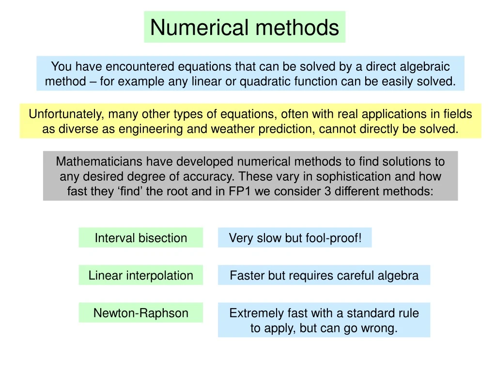
Numerical methods You have encountered equations that can be solved by a direct algebraic method – for example any linear or quadratic function can be easily solved. Unfortunately, many other types of equations, often with real applications in fields as diverse as engineering and weather prediction, cannot directly be solved. Mathematicians have developed numerical methods to find solutions to any desired degree of accuracy. These vary in sophistication and how fast they ‘find’ the root and in FP1 we consider 3 different methods: Interval bisection Very slow but fool-proof! Linear interpolation Faster but requires careful algebra Newton-Raphson Extremely fast with a standard rule to apply, but can go wrong.
Interval Bisection WB10 (a) Show that the equation f (x) = 0 has a root between x =1 and x = 2. Establish root by showing change of sign in interval Change of sign root in interval (b) Starting with the interval [1, 2], use interval bisection twice to find an interval of width 0.25 which contains From (a), function is increasing in interval [1,2]
Care must be taken establishing whether the function is increasing or decreasing Eg (a) Show that the equation f (x) = 0 has a root between x =0 and x = 1. Establish root by showing change of sign in interval Change of sign root in interval From (a), function is decreasing in interval [0,1] (b) Starting with the interval [0, 1], use interval bisection to find the correct to 1dp A decreasing function reverses the way you interpret the results so use a diagram!
GCSE recap: similar triangles The lengths of sides are multiplied by the scale factor k Eg two similar triangles x k Eg if triangles RST and UVW are similar S V Hence T R W U This property can be used to solve problems
Similar shapes Eg PQ is parallel to ST PQ = 4cm, ST = 10cm, QR = 3cm, RT = 9cm Q 4cm 3cm P ΔSRT and ΔQRP are similar as: 9cm R QPR and STR are alternate T PQR and TSR are alternate PRQ and SRT are vertically opposite 10cm Work out the length of RS S Make separate sketches Similarity R R Taking part of this statement, 3cm 9cm P Q 4cm S T 10cm
This method can be used to approximate the roots of equations by a method called linear interpolation Eg Use linear interpolation once on this interval to find an approximation to . Give your answer to 3 decimal places. The equation has a solution in the interval [1,2]. In this method, you imagine the curve to be a straight line between the limits of the initial interval, then use similar triangles to locate where this line crossed the x-axis Similar triangles So function is increasing in interval [1 , 2]
WB11 The root of the equation f (x) = 0 lies in the interval [1.6,1.8]. Use linear interpolation once on the interval [1.6, 1.8] to find an approximation to . Give your answer to 3 decimal places. As f(1.6) and f(1.8) are awkward, call their absolute values A and B to make the algebra easier and store them in your calculator’s memory So function is increasing in interval [1.6 , 1.8] Similar triangles NB: the textbook has questions which ask for solutions correct to 1 or 2dp, which could take many iterations of this method and prove incredibly awkward and time-consuming. In reality you will only be asked to ‘use linear interpolation once’ in the exam.
The Newton-Raphson Method There is a much faster method for finding roots of equations: Eg Rearrange an equation to the form f(x) = 0 Differentiate to obtain f’(x) Pick an initial solution x1 Evaluate to obtain an improved solution x2 Repeatedly applying will obtain increasingly accurate solutions etc
WB12 (a) Write down, to 3 decimal places, the value of f(1.3) and the value of f(1.4). (b) Taking 1.4 as a first approximation to α, apply the Newton-Raphson procedure once to f(x) to obtain a second approximation to α, giving your answer to 3 dp
WB13 (a) Show that f (x) = 0 has a root between 1.4 and 1.5. Change of sign root in interval (b) Taking 1.45 as a first approximation to , apply the Newton-Raphson procedure to obtain a second approximation to , correct to 3dp once to
Making your calculator do the hard work From the previous example, to solve , keep applying A scientific calculator can do this for you if you tell it at a starting value and instruct it what to do with this value repeatedly: Type ‘2 =‘ to make the Ans key x1 Then type and keep pressing =
Why does the Newton-Raphson method work? Repeating this process will ‘home in’ on the root Although much more powerful and ‘mechanical’ than the other methods, it does occasionally go wrong…
Numerical methods Eg The equation has a solution in the interval [1,2]. So function is increasing in interval [1 , 2] Interval bisection Linear interpolation Similar triangles Newton-Raphson using x1 = 2