Download
1 / 26
260 likes | 366 Views
This study focuses on integrating existing genetic data sets (EDS) with novel data collections (NDC) to identify genetic units' effects. The compound local True Discovery Rate (cℓTDR) is crucial for estimating the genetic unit’s impact accurately. Estimations involve calculating prior probabilities from EDS and combining them into a single set. By transforming all data into a common genetic unit, such as SNPs, we can achieve a standardized analysis. Understanding combined prior probabilities is essential for determining the likelihood of a test unit's significance within the NDC. The methodology outlined helps establish a rigorous mathematical foundation for genetic data integration and analysis.

E N D
Integrating heterogeneous genetic data sets based on rigorous mathematical foundation Oct 21, 2010 József Bukszár et al. Center for biomarker research and personalized medicine
et al. • Amit N. Khachane • Karolina Aberg • Youfang Liu • Joseph L. McClay • Patrick F. Sullivan • Edwin J. C. G. van den Oord
Data integration Our goal is to find test units that have effect in the novel data collection (NDC) using information from existing data sets (EDS-s) as well. Existing data set (EDS) (e.g. linkage data) Existing data set (EDS) (e.g. linkage data) Existing data set (EDS) (e.g. linkage data) Incorporation Novel data collection (NDC) (e.g. GWAS, sequencing) Compound local True Discovery Rate (cℓTDR) cℓTDRof a genetic unit is the posterior probability that the genetic unit has an effect in the NDC based on the information in the NDC and EDS-s. Genetic unit: SNP in GWAS, gene in expression data, an entire chromosomal segment in next-generation sequencing of regions of interest.
The ℓTDR ℓTDRof a genetic unit is the posterior probability that the genetic unit has an effect in the NDC based on the information in the NDC only. Novel data collection (NDC) (e.g. GWAS, sequencing) Compound local True Discovery Rate (cℓTDR) Genetic unit: SNP in GWAS, gene in expression data, an entire chromosomal segment in next-generation sequencing of regions of interest.
The compound ℓTDR (cℓTDR) The compound ℓTDR (cℓTDR) of a test unit is defined as the posterior probability that the test unit is alternative in the NDC based on the information we have from the EDS-s and the NDC: the observed statistic of test unit j in the NDC the event that test unit j is alternative in the NDC the rank of test unit j in the i-th EDS A direct consequence of the definition: the sum of the cℓTDR-s of genetic units in a group of genetic units = = the expected number of genetics units with effect in this group
Using cℓTDR / ℓTDR 10,000 genetic units with larges cℓTDR-s all genetic units the total number of gen. units with effect 5703 1822 Cumulative cℓTDR at k = the sum of the largest k cℓTDR-s = = the expected number of genetic units with effect among the k genetic units with largest cℓTDR-s. Cumulative cℓTDR at 6000 =1822.
Using cℓTDR / ℓTDR 5703 In the ideal scenario we would have 5703 genetic units with cℓTDR 1, and the rest with cℓTDR 0 (blue curve). The closer the cumulative cℓTDR/ℓTDR curve is to the blue curve, the more information we have. How can we estimate cℓTDR / ℓTDR accurately?
Estimating cℓTDR for the NDC using (combined) prior probabilities from the EDS-s The cℓTDR of a test unit j can be calculated as where j(combined prior) is the prior probability that test unit j is alternative in the NDC based on the combined information we have from all EDS-s, f0 and f1 are the null and alternative density functions (pdf) in the NDC, resp., tj is the observed statistic of test unit j in the NDC. We need to estimate/have • j(combined prior) , • f0 and f1 (pdf-s in the NDC), which we will plug in the above formula.
Test units Existing data set (EDS) (e.g. linkage data) Existing data set (EDS) (e.g. linkage data) Existing data set (EDS) (e.g. linkage data) Transformation into test unit data Transformation into test unit data Transformation into test unit data Incorporation Novel data collection (NDC) (e.g. GWAS, sequencing) Compound local True Discovery Rate (cℓTDR) First step: we transform every data set in such a way that they are based on the same genetic unit. This common genetic unit will be referred to as test unit. Example.: If the NDC is a GWAS and the EDS-s are gene expression data, then we can transform the EDS-s into SNP-based data sets. The test unit will be SNP.
Estimating the combined prior probabilities j(combined prior) Existing data set (EDS) (e.g. linkage data) Existing data set (EDS) (e.g. linkage data) Existing data set (EDS) (e.g. linkage data) Transformation into test unit data Transformation into test unit data Transformation into test unit data Prior probabilities Prior probabilities Prior probabilities Combined prior probabilities Incorporation Novel data collection (NDC) (e.g. GWAS, sequencing) Compound local True Discovery Rate (cℓTDR) • We estimate prior probabilities of test units for each EDS. • We combine the sets of prior probabilities into a single set • of prior probabilities.
Estimating prior probabilities for a single EDS Theorem: For the (prior) probability that test unit i is alternative in the NDC we have that where the contribution of test unit i from the EDS to the NDC and ri is the rank of test unit i in the EDS (r) is the probability that a test with rank r in the EDS is alternative in the EDS m1 is the number of test units alternative in the EDS m1* is the number of test units in the EDS that are alternative in the NDC m1overlap is the number of test units that are alternative in the EDS and in the NDC m is the number of test units that are in the EDS and in the NDC
Statistic for estimating the contributions We will use the test statistic where the higher the better the lower the better where tj is the NDC test statistic of test unit j and rj is the rank of test unit j in the EDS, and The above statistic can be calculated for any real number d≥0 and positive integer M.
The rationale of the statistic The idea is that the group of test units with |tj| ≥ d is likely to contain “many” test units with effect if d is large. The statistic fluctuates around 0 if the being an alternative in the EDS is independent of being an alternative in the NDC. If test units that are alternative in the NDC are more likely to be alternative in the EDS than the test units that are null in the NDC, then the statistic will be positive for small M and large d.
Stanley schiz. as EDS and 16 GWAS as NDC Stanley reshuffled Stanley Statistic values The Stanley p-values were reshuffled on the genes. M
Stanley schiz. as EDS Statistic values Statistic values M M Lower range of M Full range of M
Stanley bipolar Statistic values Statistic values M M Lower range of M Full range of M
Lewis Statistic values Statistic values M M Lower range of M Full range of M
Statistic for estimating the contributions Theorem: For the expected value of our statistic we have that where CO(M) F0 and F1 are the null and the alternative c.d.f., resp., in the NDC, i.e. Note that F0 and F1 are well-defined, i.e. they always exist, even if we do not know them.
From the previous slide: Notation It follows from the previous theorem that is an unbiased estimator of CO(M), where D is a set of positive real numbers. If there are no ties among ranks in the EDS, then we use i is the test unit whose rank is M in the EDS. to estimate the contributions co(i) for i=1,…,m, where is defined 0. The case when we have ties among ranks can be handled as well.
The co(.) is lower for test units whose rank is larger in the EDS, i.e. i is the test unit whose rank is M in the EDS. is a decreasing function of M, i.e. CO(M) is a concave function. Consequently, the estimates should follow, the same pattern, i.e. should be a decreasing function of M, i.e. CO(M) should be concave. Smoothing needs to be done. Great deal of details …
Combining prior probabilities from multiple EDS-s The combined odd of test unit i is defined as where i(combined prior) is the combined prior probability of test unit i. Under mild assumptions, for the combined odd we have that where i*j is the prior probability that test unit i is alternative based on the j-th EDS, m1(NDC) is the number of alternative test units in the NDC, and m0(NDC) = m(NDC) - m1(NDC). We replace the terms with estimates in the above formula to obtain an estimate of the combined odd.
Simulation results black: cumulative cℓTDR curve red: cumulative ℓTDR curve blue: # of test units alternative in the NDC in the top test units when cℓTDR - basedselection was used green: # of test units alternative in the NDC in the top test units when ℓTDR - basedselection was used
16 GWAS as NDC For estimating the prior probabilities, we need the null and the alternative c.d.f. (F0 and F1 ), and the number of alternative test units in the NDC. We developed a parametric method for GWAS NDC. Lambda=1.169 lambda=1.00048 p-values “corrected” by the estimated distributions Original p-values
Existing data sets used • Stanley schizophrenia expression data • Lewis linkage data • OMIM (without Schiz. DB data) • Candidate genes Schiz. Database • SLEP human mouse orthologs • NR EQTL
Black: cumulative cℓTDR curve Red: cumulative cℓTDR curve
Replication study on two GWAS Blue: empirical distribution of the cℓTDR – selected p-values Red: empirical distribution of the ℓTDR – selected p-values Light blue: empirical distribution of randomly selected p-values