Download
1 / 16
160 likes | 283 Views
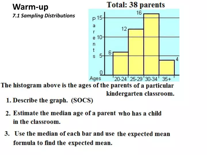
Warm-up 7.1 Sampling Distributions. Ch. 7 beginning of Unit 4 - Inference. Unit 1 : Data Analysis Unit 2 : Experimental Design Unit 3 : Probability Unit 4 : Inference. Ch. 1, 2, and 3 Ch. 4 Ch. 5 and 6 Ch. 7, 8, 9, and 10. Student of the day! Block 4. Student of the day! Block 5.

E N D
Ch. 7 beginning of Unit 4 - Inference Unit 1: Data Analysis Unit 2: Experimental Design Unit 3: Probability Unit 4: Inference Ch. 1, 2, and 3 Ch. 4 Ch. 5 and 6 Ch. 7, 8, 9, and 10
Introduction In November 2005 the Harris Poll asked 889 U.S. adults “Do you believe in ghosts?” 40% said they did. At almost the same time CBS News polled 808 U.S. adults and asked the same question. 48% of the respondents professed a belief in ghosts. Why the difference?
Sampling Distribution • Both the Harris Poll and CBS news sampled a certain number of adults for the information. Both proportions gathered are statistics and should be written as: • Imagine we have the actual parameter. And it is p = 0.45. • Both samples were not really wrong, the difference between the statistics and the parameter is called sampling error or sampling variability.
Sampling Distribution Model This is a histogram of 2000 simulations sampling 808 adults.
Characteristics of a fair sized sample • Symmetric (very Normal) • No outliers • Center p-hat will match p • The bigger the sample size the smaller the spread
The sampling distribution model In this case the p is the mean and what we normally consider the standard deviation is called the standard error. What falls in the 95% is considered reasonably likely events. Suppose we want to label the normal model with the information from the 2000 trials of 808 adults sampled about ghosts.
Assumptions and Conditions When using a sampling distribution model we need two assumptions: The Independence Assumption & Sample Size Assumption Assumptions are difficult to check. Conditions to check before using the Normal Dist. to model the distributions of sample proportions : • Randomization Condition: Applies to experiments and surveys • 10% Condition: The sample size n must be no larger than 10% of the population • Success/Failure Condition: Sample size must be big enough for at least 10 expected success or at least 10 expected failures Example: CBS poll surveyed 808 adults.
Examining a sampling distribution model The Centers for Disease Control and Prevention report that 22% of 18-year old women in the U.S. have a BMI of 25 or more – a value considered by the National Heart Lung and Blood Institute to be associated with health risk. As part of a routine health check at a large college, the physical education dept. usually requires students to come in to be measured and weighed. This year, the department decided to try out a self report system. It asked 200 randomly selected female students to report their heights and weights (from which BMI was calculated). 0nly 31 students had BMI higher than 25. How does p-hat compare to the actual proportion? (w/in SD from p) Does sampling distribution model meet the conditions? Comment on the numbers and this sampling distribution model.
Why use sampling distribution models? The textbook calls p-hat and standard error of p-hat point estimators because you use these numbers to infer something about the parameter of the population you are sampling. Just like the conditions mentioned earlier, the distribution model must produce a statistics that is unbiased and precise.
Homework/Class work • Complete E #4 and #5 4b. You can use the random # digit table in the back of the book OR Randint(1, 50) under MATH -> -> -> PRB. 5. a, d, e require making a dotplot; I expect to see these 3 dotplots