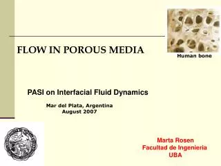
Human bone
FLOW IN POROUS MEDIA. Human bone. PASI on Interfacial Fluid Dynamics. Mar del Plata, Argentina August 2007. Marta Rosen Facultad de Ingenieria UBA. Porous media (disordered media). Motivation Environment , movement of contaminants, Oil Industry, oil recovery problems,

Human bone
E N D
Presentation Transcript
FLOW IN POROUS MEDIA Human bone PASI on Interfacial Fluid Dynamics Mar del Plata, Argentina August 2007 Marta Rosen Facultad de Ingenieria UBA
Porous media (disordered media) Motivation Environment, movement of contaminants, Oil Industry, oil recovery problems, Geological systems, Mathematical modeling of fluid flow and transport in porous media, Physical characterization of this disordered system….. Industrial, paper, textiles, graffito, carbon, cement…
Geometry has an important influence over transport besides on mechanical properties. A disordered material, can be defined because there are: *position disorder *composition disorder (coexistence of different phases: fluids in poralspace or different intrinsic properties of the material) *contact interfaces (friction ofnon consolidate grains).
Disorder Porous media are disorderly systems. Microscopic heterogeneities are at the pores of the grains (not easy observable) or in between grains… Macroscopic heterogeneities are at the level of core plugs. Megascopicalheterogeneities are at the level of the entire reservoirs (large fractures and faults). sponge
Hierarchy of heterogeneities and length scales Natural porous structures are in general heterogeneous systems. One noteworthy characteristic is their complex micro geometry . Structure: X-ray Computed Tomography Scans…
In order to analyze their structures, it is possible to make a model through the spheres or disc packing. In this way different types of compaction are obtained. 36% to 41% of free space (monodisperse) Disordered bead pack 3D 2D
First approximation: the reference of elementary solid structure forms with a single diameters spheres 47% relative free space 25% relative free space When the transport properties are studied, building an homogeneous and reproducible medium allows a better interpretation of the experimental results and their easy characterization.
However, the methods applied to ordered structures are not suitable for disordered structures (Voronoi polyhedrons where the number of polyhedrons with the same number of side are counted) . We introduce *Mean coordination number (average of contacts around one sphere) *Coordination number i (for i components) Definitions independent from the size of the sample.
Geometrical Properties Porosity Where the pore volume (Vp) denotes the total volume of the pore space in the matrix and the matrix volume (V m) is the total volume of the matrix including the pore space. The porosity has to be averaged over many pores and the considered matrix volume must be larger than the pore size. Often the porosity can be chosen as constant for the whole medium.
Adsorption experiments with N and Hg, in activated carbon porous samples Valid between 200 and 10000A (Drazer et al. )
REV Region where the parameters are defined.
Empirical relationship (Caquot 1915) Ri and Rj pores sizes Other geometrical parameters The tortuosity (T) is defined as the relationship between the mean effective length (Le)of an element of fluid volume when it crosses the porous medium and the length of the porous media (L). The element of fluid volume follows the path opened by the interconnected pores. Brain tissue
DARCY Law (1856) At the first order of approximation, the slow steady-state flow (low Re) of an incompressible fluid through a porous media is described at the macroscopic scale by the Darcy’s law. Considering the pressure p constant at the pore scale and the fluid is Newtonian. where: k = Permeability, Darcy dp/dx= Pressure gradient, atm/cm A = Cross sectional area, cm2 = Viscosity of the fluid, centipoise Q = Volumetric flow, cm3/s k is the permeability (1D=10-12 m2) Laminar flow!
The permeability of a porous medium, is a measure of how easily a fluid can flow through the medium. IMPORTANT: pm model. Some examples 2D
3D There are some models that correlated permeability with tortuosity. Archie Law Kozeny-Carman
In actual media In same regions, we can found up a broad variation of this property: from high permeability to impermeable regions Examples Unconsolidated sands may have permeability of over 5000 mD. Rocks with permabilities significantly lower than 100 mD Cretaceous rock.
Michigan Environmental Education CurriculumGroundwater Supply (Percolation)
Two types of models to analyze permeability: -Continuous (classical engineering approach), and -discrete, characterized by several length scales. Permeability as a percolative phenomena f>fcr K=0 Where fcr is the critical porosity when K=0 Wood
Experimental Model Numerical model Three-dimensional pore space of Berea sandstone [B. Biswal et al.,1998] A glass grain made up by microspheres of sintered glass is shown.
Transport or flow phenomena Dispersion Phenomena Influenced by: • Molecular diffusion • Disordered or random geometry • Velocity gradients Tracer dispersion measurements are a powerful tool for the study the behavior of flow. Different experimental methods are used to characterize the flow, and the fluid-fluid and fluid-porous interactions.
Visualization of the diffusive behavior as a function of time Dx=Ut Miscible fluids, without interfaces
Profile Evolution as a function of time in a porous medium Step function is injected Characteristic times: Dt is a mixing time t is a transit time
This mixing process is affected by the morphology of the porous structure. If those two fluids are flowing, hydrodynamic dispersion takes place and such a phenomenon can be modeled by the one-dimensional convective-diffusion equation: macroscopic eq. where x is the flow direction V is the macroscopic mean velocity C (x,t) is the macroscopic mean concentration is the Laplacian in transverse directions DL is the longitudinal dispersion coefficient DT is the transversal dispersion coefficient DT<DL
Different regimes of tracer dispersion can be identify using the a dimensional Peclet number, which is the ratio between the typical time for diffusion l2/Dm and the typical time for convection l/U. Where l is taken as the grain average diameter . Here, U is the velocity of the carrier fluid; l, a characteristic length scale of the porous media; and Dm, the molecular diffusivity coefficient of the tracer. Porous ceramics
In a disordered medium the tracer follows the streamlines. In a random walk picture, a tracer particle following the direction of the velocity field may be modeled, with steps of length l and duration equal to l/v ( ). The dispersion regimes are: -In the small Peclet number regime, molecular diffusion dominates the way in which the tracer flows. -In the large Peclet number regime, also called “mechanical dispersion”, convective effects are significant; the tracer velocity is approximately equal to the carrier fluid velocity, and molecular diffusion plays little role.
adimensional longitudinal dispersion vs Peclet number Saffman model (1959) Pe>105 Turbulent dispersion m=1 m=1.2 m=0 Pe 0.5 DL/Dm = Cte. 0.5<Pe< 5 DL U2 5<Pe< 300 DL=Ul logPe Pe300 DL= Ul
The Saffmansimplified model is in agreement with many experimental results (corresponding to capillars randomly interconnected). Where a is a porous ratio and l the length
What kind of concentration profile can we expect? Under the boundary conditions: C(x,0) = 1 for x 0 C(x,0) = 0 for x > 0 For long enough porous media (zero concentration at infinite),the solution is: The dispersion coefficient DL is obtained by fitting the variation of the concentration as a function of position (x) and time (“Gaussian” solution).
Injecting a step function of tracer Mixing zone
Concentration normalized at four sections (3, 6, 9,11 cm from inlet) obtained through measurements of activity of tracer, and at the outlet (obtained through conductivity measurements) as a function of t*. t*=tQ/Vp Symbols correspond to values obtained experimentally, and lines, their fittings.
Anomalus dispersion (tails) (non-Fickian) behavior Anomalous dispersion refers to concentration profiles that exhibit long-time tails as opposed to normal or Gaussian dispersion, which does not exhibit such tails. Laboratory and field measurements of dispersivity show a dependence on scale size and travel distance, indicating a failure of Fick's law for dispersion. The theoretical explanation can be found on the basis of mathematical models and numerical simulation studies. As the flow moves through longer distances, it encounters new heterogeneities of the media properties and from the flow resistance it encounters. Beyond this, the flow will encounter heterogeneities of increased scale size, a fact which is inconsistent with the assumptions adopted for the derivation of Fick's law, and a constant dispersivity. As a result, the flow displays a dispersivity which increases with travel distance, also known as anomalous dispersion.
Laboratory example of an a poor fitting. n = 0.8 Pe = 55 Scleroglucane Experimental results and Gaussian fits.
Other phenomenon: Trapping phenomenon
Heterogeneities Dispersivity as a function of Pe number . Simple porosity media (d = 200 m). Double porosity media ( +int = 30% (dg = 550 m, db = 55m), x . int = 30% (dg = 550 m, db = 110m).
Immiscible fluids • We need to consider the interrelationship between: • capillary effects • viscous effects • wettability, … • convective effects Two type of process -imbibitions -drainage (percolation) critical parameters
Viscosity: when a polymeric solution flow Rheological properties dV/dy is the deformation velocity of the fluid
No Newtonian fluids 0 n 1 “shear thinning” Xanthane
Carreau Xanthane
Scleroglucan Rheological curves (n=0.4, 0.55, 0.62, 0.73 and 0.77).
Velocity profiles for a N and a n-N shear thinning solution in a capillary tube.
Viscoelasticity behavior Elastic behavior of polymer solution at the capollary outlet. Newtonian Viscoelastic
The rheological index influence on the concentration profile. =41%.Péclet 57 (fluid: Scleroglucane) d=1mm (D’Onofrio)
Instabilities in porous media • Description of instabilities controlled by: • Gravity • Viscosity
Instabilities = 2+ (1-2)c = 0(1-c) is a lnear function of concentration Used relationship = (1-2)/ 2 0=2, Volume, mass and momentum conservation presión p Vx, Vy y Vz; Fourier decomposition mi1=mi1(z,t)eikx et
We introduce perturbation in velocity components and substitute pressure: Where R= . Expansion of volume coefficiant Finally =
With solution Relation of dispersion v1 = D = 0 If . Destabilizing g (R>0, Rayleigh-Taylor; R<0, dispersion eq. for gravitational wave) If =-Dk2 g = 0, Destabilizing D If g and D are different from zero Small l Large l