Download
1 / 22
220 likes | 365 Views
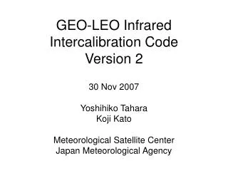
Follow-Up Review of GEO-LEO Intercalibration. 12-14 June 2007 Yoshihiko Tahara Koji Kato Ryuichiro Nakayama Toru Hashimoto Meteorological Satellite Center Japan Meteorological Agency. Intercalibration Algorithm Ver 0.0 (Delivered on May 5). LEO FOV at nadir. GEO pixel.

E N D
Follow-Up Review of GEO-LEO Intercalibration 12-14 June 2007 Yoshihiko Tahara Koji Kato Ryuichiro Nakayama Toru Hashimoto Meteorological Satellite Center Japan Meteorological Agency
Intercalibration Algorithm Ver 0.0(Delivered on May 5) LEO FOV at nadir GEO pixel • Key match-up conditions between GEO and LEO • Difference of observing times < 1800 (sec) • Difference of 1/cos( sat. zenith angles ) < 0.05 • Environment uniformity check • To choose only spatially uniform area to alleviate navigation error, MTF, observing time difference, optical path difference, etc. • Environment domain = 11x11 IR pixel box (MTSAT-1R vs. AIRS) • env_stdv_tb < (TBD) • Representation check of LEO-size GEO pixels in the environment • z-test • LEO FOV = 5x5 IR pixel box (MTSAT-1R vs. AIRS) • abs( fov_mean_tb – env_mean_tb ) < Gaussian x env_stdv_tb / 5 LEO-size box 5 x 5 pixels Environment box11 x 11 pixels
2-D Density distributionbetween SD and MEANof 10.8-micron TBsin 11x11-pixel boxover MTSAT-1R SSP region (coloered by log scale) 10.8-micron S.D. of TBs [K] S.D. of TBs [K] MEAN of TBs [K]
2-D Density distributionbetween SD and MEANin 11x11-pixel boxover MTSAT-1R SSP region 6.8-micron S.D. of TBs [K] 3.8-micron MEAN of TBs [K] S.D. of TBs [K] MEAN of TBs [K]
2-D Density distributionbetween SD and MEANof 10.8-micron Radiancesin 11x11-pixel boxover MTSAT-1R SSP region 10.8-micron S.D. of Rad [W/cm^2.sr.um] TB density Radiance density d Rad / d TB @ 300 K S.D. of Rad [W/cm^2.sr.um] MEAN of Rad [W/cm^2.sr.um]
6.8-micron Radiance TB d Rad / d TB @ 250 K S.D. of Rad [W/cm^2.sr.um] 3.8-micron Radiance TB d Rad / d TB @ 300 K S.D. of Rad [W/cm^2.sr.um] MEAN of Rad [W/cm^2.sr.um]
Expectation Number of LEO-FOV Boxes Passing Uniformity and Representation Checks in 1 Scene 10.8-micron 6.8-micron 3.8-micron Criterion of Uniformity Check • Notes: • The criterion of z-test for the representation check of LEO-FOV (GEO 5x5-pixel box) is 95 %. • The number of LEO-FOV boxes passing time and SZA difference checks is assumed to be 30000 at one GEO-LEO co-location scene. • The results only represent over the West Pacific Tropical region.
TB Test and Radiance TestCase Study at 16 UTC, Feb 21 Radiance test SD ~ 2 K @ 300 K Z < 0.95 % N = 1809 10.8-micron TB of MTSAT-1R [K] TB test SD ~ 2 K Z < 0.95 % N = 1567 w/o tests TB of AIRS Constrained Virtual Channel [K] Radiance test SD ~ 2 K @ 300 K Z < 0.95 % N = 2720 3.8-micron TB of MTSAT-1R [K] TB test SD ~ 2 K Z < 0.95 % N = 1731 w/o tests TB of AIRS Constrained Virtual Channel [K]
TB Test and Radiance TestCase Study at 16 UTC, Feb 21 TB difference between MTSAT-1R IR1 (10.8-micron) and AIRS virtual channel (constrained) 10.8-micron 10.8-micron TB test SD ~ 2 K Z < 0.95 % N = 1567 Radiance test SD ~ 2 K @ 300 K Z < 0.95 % N = 1809
TB Test and Radiance TestCase Study at 16 UTC, Feb 21 TB difference between MTSAT-1R IR4 (3.8-micron) and AIRS virtual channel (constrained) 3.8-micron 3.8-micron TB test SD ~ 2 K Z < 0.95 % N = 1731 Radiance test SD ~ 2 K @ 300 K Z < 0.95 % N = 2720
Radiance Comparison and TB Comparison Radiance Residual TB Residual 3.8-micron 3.8-micron Radiance test SD ~ 2 K @ 300 K Z < 0.95 % N = 2720 d Rad / d TB @ 300 K
TB Comparison and Radiance Comparison d Rad / d TB @ 300 K 10.8-micron Radiance of MTSAT-1R minus AIRS Radiance of MTSAT-1R Radiance of AIRS Constrained Virtual Channel [W/cm^2.sr.um] TB comp. Radiance comp. d Rad / d TB @ 300 K 3.8-micron Radiance of MTSAT-1R minus AIRS Radiance of MTSAT-1R Radiance comp. TB comp. Radiance of AIRS Constrained Virtual Channel [W/cm^2.sr.um]
Review of Algorithm Ver 0.0 • Environment and representative checks should be examined in radiance space rather than TB space • Radiance criteria of the environment and representative checks depend on channels, but they can be the same over clear and cloudy regions • Radiance comparison between LEO and GEO should be computed • Or the results should be converted to calibration parameters
Constrained Virtual Channel Radiance observed by a broadband channel is Radiance of a virtual channel (linear combination of HSRS radiances) is They should be approximately equal for any I(v), then To obtain wi, solve where
Convolution and Constrain Methods 12.0-micron
Convolution and Constrain Methods (w/ gaps) 10.8-micron 6.8-micron
Blacklisted Channels and Gaps • Blacklisted channels and the AIRS observing gaps yield the unstable SRF of a virtual channel • The unstable weights of the virtual channel are not proper for the use of real HSRS observations that contain observing errors # of blacklisted AIRS channels is 41in MTSAT-1R IR2 observing range(790 cm-1 – 880 cm-1)
Review of Constrained Virtual Channel • Without gaps and blacklist channels in HSRS over a GEO channel region, the constrain method is better than the convolution method • If there is a gap, the advantage of the constrain method becomes unclear. In this case, the key is how to fill the gap correctly • Removing HSRS blacklist channels from computing the SRF of a constrained virtual channel makes the SRF unstable.
Experiment of Visible ComparisonMTSAT-1R vs. NOAA-18/AVHRR Comparison of Reflectance • Match-up conditions: • d Time < 10 min • d Pos < 0.8 km • d sec( SZA ) < 0.05 • d LookAngle < 2 deg • No uniformity check
Experiment of Visible ComparisonMTSAT-1R, 2 vs. RSTAR6 MTSAT-1R MTSAT-2 • Radiative Transfer Simulation • RSTAR6 RT code provided by Prof. Nakajima et al, Tokyo Univ. • Atmospheric state: JCDAS (JMA climate data assimilation system, extended run of JRA-25) • Aerosol and cloud: MODIS products released by NASA • Ozone: Aura/OMI product released by NASA
Artificial Channels to Fill AIRS Gaps . . . . . . . . . . . AIRS SRFs • SRFs of “Artificial channels” • Gaussian curve (sigma = 0.5 cm-1) • Intervals = 0.5 cm-1 SRF of AIRS virtual channel w/o artificial channels Using artificial channels