
Linear Programming: The Carpenter's Problem in Standard Form
E N D
Presentation Transcript
CS 575Design and Analysis ofComputer AlgorithmsProfessor Michal CutlerLecture 20April 18, 2005
This class • The problem • Graphical solutions • Standard and slack forms • The simplex algorithm • Finding an initial feasible solution
Linear Programming • Among most important advances of 20th century • Generalizes many classical problems • Shortest path, max flow, multi-commodity flow, MST, traveling salesman • Often used for optimal allocation of scarce resources • Helps to find “good” solutions to NP-hard optimization problems
The carpenter’s problem • A carpenter manufactures 2 types of tables. • Production is limited because of availability of labor, glass and wood.
Profits • Only round tables – 10 with profit of $700 • Only rectangular tables – 10 with profit of $900 • 5 round and 8 rectangular – 5*70 + 8*90= $1070
Standard form for LP • Note that the objective function and the inequalities are linear
The carpenter’s problem in standard form • In the following slides we solve the problem using geometry • Show feasible region and extreme points
Feasible regionfor carpenter problem Rectangular table Glass 5x+3y=50 (0, 10) (5, 8) Labor 3x+2y=31 (7, 5) Feasible region Wood 4x+10y=100 (0,0) (10,0) Round table
Objective function70x+90y Rectangular table Profit (0, 10) (5, 8) 70x+90y=$700 (7, 5) Feasible region 70x+90y=$1070 (0,0) (10,0) Round table
Integer linear programming • The carpenter’s problem requires integer solutions • Typically linear programming algorithms do not produce integer solution! • Integer programming in NP-hard!
(0, 10) (5, 8) (7, 5) LP:Geometry Rectangular table Extreme Points of feasible region (0,0) (10,0) Round table
LP: Geometry in general • The solutions of a linear program form an n-dimensional convex polyhedron • Convex : if y and z are feasible solutions, so is ay + (1 - a)z where 0<a<1 • When the solutions of a problem are a convex set and the object function is convex on the convex set a localoptimal solution is a global one • No need to worry about local optima!
LP: Geometry in general • Extreme point: vertex of the polyhedron (solution cannot be expressed as a linear combination of two different solutions y and z satisfying ay + (1 - a)z where 0<a<1) • Extreme point theorem: If there exists an optimal solution to standard form LP, then there exists one that is an extreme point • Need to consider only a finite number of solutions
LP: Main idea of the simplex algorithm • Main idea of the simplex algorithm: search for optimal solution by moving from one extreme point of the polyhedron to a neighboring extreme point without decreasing the objective function
George Danzig – invented Simplex algorithm • First algorithm for solving linear programming problems. (Danzig 1947) • Developed after WWII in response to logistic problems • Used for 1948 Berlin airlift • Finite (exponential) complexity
A “large scale” problem • The first "large-scale" problem was a 9 by 77 instance of the "diet problem" (find a min-cost diet that meets or exceeds nutritional requirements), solved by 9 clerks using hand- operated desk calculators, in about 120 man-days. • Current problems solved with thousands of unknowns and inequalities
Polynomial algorithms • Ellipsoid (Khachian 1979, 1980) • Resolved question of whether linear programming is NP-hard (it is not) • Not practical algorithm • Karmarkar’s algorithm (1984) and other interior point algorithms • Competitive with simplex • Likely to dominate on large problems
Transforming to standard form (1) • Often a linear programming problem is not in standard form • Inequality with (multiply by –1) x+5y-6z22 -x-5y+6z-22 • Equality = (transform to one inequality with , and one with ) x+5y-6z=22 x+5y-6z 22 and (from x+5y-6z 22 to) -x-5y+6z -22
Transforming to standard form (2) • Objective function is minimum Multiply by –1 and replace by maximum min x+5y-6z max -x-5y+6z • x is unrestricted Replace x in problem by y-z, and add y0, z0 After finding the optimal solution x can be calculated as y-z. If y z in the optimal solution then x 0, otherwise if y < z in the optimal solution then x < 0.
Transforming to standard form (3) • x c for c < 0 for example x -3 Replace x in problem by -y + c, add y0 After finding the optimal solution, x can be calculated as –y+c.Since y0, x c is satisfied in optimal solution
Slack form • Given • We introduce a slack variables and rewrite the inequality as: and add • Apply this conversion to each constraint
Example – converting to slack form • B = {x4, x5, x6} set of basic variables • N = {x1 , x2, x3} set of nonbasic variables
The simplex algorithm • For this example slack form provides a basic feasible solution: (0, 0, 0, 30, 24, 36) and z = 0 • To increase z select a nonbasic variable xe whose coefficient in z is positive and increase xe as much as possible without violating the constraints
The simplex algorithm (1) • For this example slack form provides a basic feasible solution: (0, 0, 0, 30, 24, 36) and z = 0 • To increase z select a nonbasic variable xe whose coefficient in z is positive and increase xe as much as possible without violating the constraints
The simplex algorithm (2) • This non basic entering variable xe will now become basic and another variable xl non basic. • Let x1 be the selected entering variable • From (1) 0 x4= 30 - x1 x1 30, • From (2) 0 x5= 24 - 2x1x1 12, • From (3) 0 x6= 36 - 4x1 x1 9. • Equation (3) causes the tightest limitation on x1. So x6 is the leaving basic variable
The simplex algorithm (3) • From equation (3) we get: x1 =9-x2 /4-x3/2- x6 /4 • Substituting x1 in (0), (1) and (2) we get:
The simplex algorithm (4) • Select x3 as new basic variable • From 0 x1= 9 - x3/2x3 18, • From 0 x4= 21 – 5x3/2 x3 42/5 • From 0 x5= 6 - 4x3 x3 3/2. • So x5 is the new non basic variable
The simplex algorithm (5) • From the equation for x5 (3’) we get: x3 = 3/2-3x2/8-x5/4+x6/8 • Substituting x3 in the equations (0’,1’ and 2’) for x1 and x4, and z we get:
The simplex algorithm (6) • Select x2 as new basic variable • 0 x1= 33/4 - x2/16x2 132, • 0 x3=3/2 – 3x2/8 x2 4 • 0 x4= 69/4 + 3x2/16x2. • So x3 is the new non basic variable
The simplex algorithm (7) • The optimal solution is (8, 4, 0,18,0,0), z=28 • The value of x4 =18 is the slack between the left side x1+ x2 = 12 of the original inequality x1+ x2 + x330, and the right hand side 30
In Summary: • The entering variablexe is one for which the coefficient ce in z is positive. • The leaving variable is the one that causes the tightest constraint on the entering variable. • If the tightest constraint on the entering variable is infinity, the linear program is unbounded
Unbounded solution example • Let x1 be the entering variable • From (1) and (2), x1 infinity • So x1 can be increased to infinity and solution is unbounded
Graphical solution -x1+x2 =2 -2x1+x2 =1 x2 (1, 3) Feasible region (0, 1) (0,0) objective function x1+2 x2 =5x1
Termination • It is easy to see that no iteration of the algorithm decreases the objective function • Unfortunately, the objective function may remain unchanged. This phenomenon is called degeneracy
Example Next iteration when x2 becomes basic the objective function will grow to 16
Cycling • Simplex cycles if the slack forms at two different iterations are identical (since it is a deterministic algorithm it will cycle through the same series of slack forms forever.) • There are various rules to avoid cycling • Bland’s rule: always choose the variable with the smallest index (for entering the one with the first positive c, for leaving the first most restricting variable)
Finding an initial basic feasible solution • When there are negative b values in standard form the corresponding slack form is not feasible • Let L denote the original problem • To find an initial feasible solution to L if it exists we formulate an auxiliary problem Lmax
Simplex when initial solution not feasible • Formulate an auxiliary problem Lmax • Transform basic solution to make it feasible • Use Simplex to find an optimal solution to Lmax • If solution <0 there is no feasible solution to original problem L • Otherwise in the optimal solution of Lmax: • Substitute the objective function by the objective function of the original problem L after substituting in it all variables that are basic in the optimal solution of Lmax. • Eliminate x0 from the constraints • Apply Simplex to find an optimal solution to original problem L
1.The auxiliary problem Lmax • L is feasible iff the optimal solution for Lmax is 0 • If L is feasible, combine the feasible solution with x0 = 0 resulting in a feasible solution to Lmax. Since z=0 solution is also optimal • If the optimal solution of Lmax is 0, the solution without x0 = 0 is feasible for L • Conclusions: If the solution for Lmax is not 0 L is not feasible. If the solution for Lmax is 0 we now have a feasible solution for L
2.Transform basic solution to make it feasible • Since there are negative b values, the current solution is not feasible • Choose the variable xs with the smallest value in the basic solution as the leaving variable, and x0 as the entering one • It is easy to prove the new solution is feasible