Download
1 / 10
100 likes | 195 Views
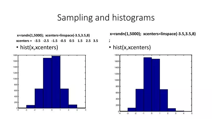
Sampling and histograms. x= randn (1,5000); xcenters = linspace (-3.5,3.5,8) xcenters = -3.5 -2.5 -1.5 -0.5 0.5 1.5 2.5 3.5. x= randn (1,5000); xcenters = linspace (-3.5,3.5,8) ;. hist ( x,xcenters ). hist ( x,xcenters ). More boxes. x= randn (1,5000);

E N D
Sampling and histograms x=randn(1,5000); xcenters=linspace(-3.5,3.5,8) xcenters = -3.5 -2.5 -1.5 -0.5 0.5 1.5 2.5 3.5 x=randn(1,5000); xcenters=linspace(-3.5,3.5,8) ; hist(x,xcenters) • hist(x,xcenters)
More boxes • x=randn(1,5000); • hist(x,20) • x=randn(1,5000): • Hist(x,20) )
CDF with only 500 samples z=randn(1,500);[f,x]=ecdf(z); plot(x,f); hold on X=[-4:0.1:4];p=normcdf(X,0,1);plot(X,p,'r'); xlabel('x'); ylabel('normal CDF') Repeat z=randn(1,500);[f,x]=ecdf(z); plot(x,f); three more times
Probability plot • z=randn(1,500); probplot(z) • Repeat (hold off)
Lognormal distribution • Mode (highest point) = • Median (50% of samples) • Mean = • Figure for =0.
Lognormal probability plot z=lognrnd(0,1,1,500);probplot('lognormal',z) probplot(z)
The normalizing effect of averaging z=lognrnd(0,1,100,500); zmean=mean(z); probplot(zmean) mean(zmean') =1.6395 %Exact mean=exp(0.5)= 1.648 std(zmean')= 0.2088 %Original standard deviation=sqrt(exp(1)-1)*exp(1))=2.1612
Fitting a distribution x=randn(20,1)+3; [ecd,xe,elo,eup]=ecdf(x); pd=fitdist(x,'normal') pd = NormalDistribution Normal distribution mu = 2.89147 [2.36524, 3.41771] sigma = 1.1244 [0.855093, 1.64226] xd=linspace(1,8,1000); cdfnorm=normcdf(xd, 2.89147, 1.1244); plot(xe,ecd,'LineWidth',2); hold on; plot(xd,cdfnorm,'r','LineWidth',2); xlabel('x');ylabel('CDF') plot(xe,elo,'LineWidth',1); plot(xe,eup,'LineWidth',1)
Fit lognormal instead pd=fitdist(x,'lognormal') pd = LognormalDistribution Lognormal distribution mu = 0.973822 [0.759473, 1.18817] sigma = 0.457998 [0.348303, 0.668939] cdflogn=logncdf(xd,0.973822,0.45799); hold on; plot(xd,cdflogn,'g','LineWidth',2)
With more points it is clearer Same as before, but with 200 points x=randn(200,1)+3; [ecd,xe,elo,eup]=ecdf(x); pd=fitdist(x,'normal') Normal distribution mu = 3.00311 [2.87373, 3.13248] sigma = 0.927844 [0.844952, 1.02891] pd=fitdist(x,'lognormal') Lognormal distribution mu = 1.04529 [0.996772, 1.09382] sigma = 0.347988 [0.3169, 0.385893]